Diversity Subset Selection on Lines and Staircases

My report, titled Exact Dynamic Programming for Solow–Polasky Diversity Subset Selection on Lines and Staircases, is now available on arXiv: https://arxiv.org/abs/2604.26929.

In multiobjective optimization and decision analysis, we often face a deceptively simple task: from a larger set of candidate solutions, choose a smaller subset that is still representative, well-spread, and diverse. This sounds easy when the points are drawn on a line or a curve. But as soon as we ask for a precise mathematical objective, the problem can become combinatorially difficult.

My new arXiv report studies such a subset selection problem for the Solow–Polasky diversity measure, introduced by Andrew Solow and Stephen Polasky in their work on measuring biological diversity. The measure was originally motivated by biodiversity, but the mathematical idea is much broader: a set should be considered diverse when its elements are mutually dissimilar. In the report, this dissimilarity is represented through a metric distance between points and an exponential similarity kernel.

A major source of inspiration for me was Tom Leinster’s beautiful book Entropy and Diversity: The Axiomatic Approach. Leinster develops a broad mathematical view of diversity, entropy, similarity, and magnitude, showing how ideas from biodiversity lead naturally to deep questions in mathematics. My note is much narrower and algorithmic in scope, but it is written in the same spirit: diversity is not merely a verbal concept. It can be formalized, studied, and optimized.

The general optimization problem is hard, but the report identifies some structured geometric cases where exact dynamic programming is possible. The pleasant surprise is that these cases are not limited to points on a line. They also include certain monotone staircases in the , or Manhattan, metric.

This result because it connects several ideas: diversity measures, dynamic programming, ordered sets, Pareto fronts, the geometry of the norm (taxi-cab, Manhattan distance), and the older max–min diversity criterion. It also gives a nice geometric picture: exact algorithms become possible when the point set can be walked through like an ascending staircase.

The problem: choosing a diverse subset

Suppose we have a finite ordered list of points and we want to choose exactly of them. The points might be candidate solutions of a multiobjective optimization problem, designs generated by an algorithm, or representative scenarios in a decision-support model.

A classical way to measure diversity is to use the Solow–Polasky diversity measure. Very roughly speaking, this measure assigns higher value to sets whose elements are less similar to each other. In the setting of the report, similarity is modeled by the exponential kernel , where is the distance between two selected points and the positive parameter controls how quickly similarity decays with distance.

If two points are close, their similarity is large. If they are far apart, their similarity is small. The Solow–Polasky value is then computed from the inverse of the similarity matrix. In this way, the diversity of a set is not just a count of its elements, but also reflects how different the elements are from each other.

This sounds like a natural diversity metric, and as for instance Solow and Polasky, as well as Leinster has shown, it has also many nice mathematical properties, which distinguishes it from other ways to measure diversity; but it is not obvious how to optimize it. For arbitrary finite metric spaces or arbitrary point sets in the plane, the problem is computationally difficult. The question is therefore: are there meaningful geometric situations where the optimal subset can be found exactly and efficiently? The answer in the report is yes.

First warm-up: points on a line

The cleanest case occurs when the points are ordered on a line, say as . In this case, the Solow–Polasky diversity of a selected ordered subset has a remarkable structure. If the selected points are , taken in increasing order, then the diversity value depends additively on the consecutive gaps.

A compact way to write the gap reward is . The full value is one plus the sum of these rewards over consecutive selected gaps. This is the key observation: on the line, the objective decomposes into local contributions. The contribution of moving from one selected point to the next depends only on the gap between them. A detailed proof for the Solow Polasky Diversity of this essential property is provided in my report.

Once we have such a decomposition, dynamic programming enters naturally. The Bellman recursion asks: what is the best value of an -point chain ending at point ? If the previous selected point is , then the last contribution is the gap term from to .

The recursion computes by maximizing over predecessor indices. This is a familiar dynamic-programming pattern: solve all smaller problems, then append the last point. The result is an exact algorithm with running time .

Figure 1 illustrates this idea for a small ordered set of points on a line. The blue points are the available candidate points. The red points show the selected subset returned by the exact dynamic program. In this example, the selected points are well balanced along the line, and the red distance markers indicate the consecutive gaps that contribute to the Solow–Polasky value. This already gives some intuition: for a concave increasing gap reward, spreading selected points rather evenly is beneficial.

From lines to Pareto fronts

The next step is more interesting for multiobjective optimization. Many Pareto-front approximations in two objectives have an ordered structure. For an optimization problem with two objectives, as one objective improves, the other gets worse. We may have points with and .

In the Euclidean metric this does not immediately reduce to a line problem. But in the metric, something simple and beautiful happens. Whenever point comes before point in the ordering, . If we define a transformed scalar coordinate , then .

So the ordered two-dimensional Pareto front has exactly the same distance matrix as an ordered set of points on a line. This is the reason why the same dynamic program applies.

This is the first staircase picture. A path from one point to another on such a front can be drawn as a right-angle polyline: move horizontally, then vertically. Its length is the Manhattan distance. The geometric curve is two-dimensional, but the ordered distances behave like distances on a line.

Figure 2 shows such a planar Pareto-front example. Again, the blue points are the full set of candidate points. The red boundary circles indicate the selected subset. The dashed staircase is not meant as a Euclidean curve connecting the points. It is the path the length of which is the distance between points: a sequence of horizontal and vertical moves whose total length equals the Manhattan distance. In the example, the selected red points split the total staircase length into two equal consecutive gaps, which is optimal for the displayed parameter choice.

A random Pareto-front illustration

The report also includes a larger random example on a simple nonlinear Pareto-front curve. Here the purpose is not to claim that all Pareto fronts are easy. Rather, the example shows how the ordered structure can still make the dynamic program applicable in a visually meaningful setting.

The selected points are not found by a heuristic. They are obtained by the exact Bellman recursion. This is important: once the ordered-distance decomposition is valid, the dynamic program compares all possible predecessor choices implicitly and returns a globally optimal subset.

Figure 3 gives this larger illustration. The blue points again represent the full candidate set sampled along the front. The red points show the subset selected by the exact algorithm. Visually, the red points form a smaller and well-spaced representation of the larger blue point cloud. Mathematically, however, this is not just an aesthetic choice: the guarantee comes from the ordered distance structure and the Bellman recursion.

The new geometric extension: monotone staircases

The report then takes one further step. The same idea is not restricted to two dimensions. Consider a finite point set . Suppose that the points can be reindexed so that the same ordering sorts all coordinate projections: for all coordinates .

Then the points form a chain in the coordinatewise partial order. Geometrically, we can walk from one point to the next using axis-parallel moves without ever moving backwards in any coordinate. This is what I call a monotone staircase.

For consecutive or nonconsecutive points in such an ordering, the distance is again just a difference of scalar potentials. Define . Then, for two points in this order, .

This reduces the monotone staircase to the line case. Hence the same Solow–Polasky dynamic program remains exact.

The report also allows the slightly more general signed version: some coordinates may be reversed first. This is useful for Pareto-front settings, where one objective may increase while another decreases. After flipping the signs of suitable coordinates, the points become coordinatewise monotone.

Figure 4 shows a three-dimensional example. The staircase starts at and moves by right-angle steps through points such as , , and . The marked points are placed directly on the staircase. The three coordinate directions are drawn in different colors: one color for motion in the first coordinate, one for motion in the second coordinate, and one for motion in the third coordinate. The light-gray projections onto coordinate planes are visual aids. They help the reader see where the three-dimensional points sit when projected down onto lower-dimensional coordinate views.

This is perhaps the most geometric part of the report. The dynamic-programming result is really about an ordered metric structure, but the staircase picture makes the condition easy to remember: if the points can be walked through monotonically, without backtracking in the relevant coordinate directions, then the distances behave like distances on a line.

A comparison: max–min diversity

The report also comments on another classical diversity objective: the minimum pairwise distance, sometimes called max–min diversity. Here one chooses a subset that maximizes the smallest distance between any two selected points. If is the selected subset, this smallest distance is the bottleneck value .

This objective has a related dynamic-programming structure on ordered sets. It is not additive over gaps in the same way as the Solow–Polasky expression above. Instead, it has a bottleneck or subadditive structure. On a line, the relevant recursion uses the two quantities and : one keeps the smaller of the two as the new bottleneck, and then chooses the predecessor giving the largest bottleneck.

So the last step does not add a reward. It updates the current bottleneck by taking a minimum. The dynamic program then chooses the predecessor that maximizes this bottleneck. The structure is different, but it is again exact because the ordered geometry reduces the problem to consecutive gaps.

This max–min objective is also closely related to Riesz-energy subset selection. In fact, max–min diversity can be viewed as a limiting case of Riesz -energy as . Informally, as the exponent grows, the smallest selected distance dominates the energy. This connection appears in related work by Pereverdieva et al. and in my earlier arXiv note on dynamic programming ideas for Riesz-energy subset selection.

The contrast is useful. Solow–Polasky diversity on ordered exponential-kernel line metrics leads to an additive sum of transformed gaps. Max–min diversity leads to a bottleneck recursion. Riesz-energy subset selection lies nearby, but the exactness of simple recursions depends more delicately on the objective.

Outlook

The report leaves also some questions open. Can similar exact recursions be found for other diversity measures? Can the dynamic program be accelerated for larger ordered instances? Can useful approximation methods be designed for point sets that are close to, but not exactly, monotone staircases?

Another natural direction is to study higher-dimensional Pareto fronts more systematically. The staircase condition is strong: it requires a single ordering, possibly after sign changes, that sorts all coordinate projections. General Pareto fronts in three or more objectives will not usually satisfy this. But they may contain monotone chains, or they may be decomposable into chain-like pieces.

This is where I think the geometric picture becomes useful. Instead of asking only whether a subset selection problem is hard or easy in full generality, we can ask: which geometric structures make exact optimization possible?

For the Solow–Polasky diversity measure with the exponential kernel and the metric, lines and monotone staircases provide one answer.

Report

The arXiv report is titled Exact Dynamic Programming for Solow–Polasky Diversity Subset Selection on Lines and Staircases. It contains the formal statements, proofs, examples, and the dynamic-programming algorithm (as a python listing). The examples include the one-dimensional case, planar Pareto fronts, and a three-dimensional staircase illustration.

Read the report on arXiv: https://arxiv.org/abs/2604.26929

References

T. Leinster, Entropy and Diversity: The Axiomatic Approach, Cambridge University Press, 2021.

A. R. Solow and S. Polasky, “Measuring biological diversity,” Environmental and Ecological Statistics, 1, 95–103, 1994.

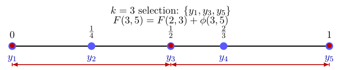
Figure 1: A diverse subset is chosen from all blue points on the line and marked in red. Also, a single step in the Bellmann recursion is highlighted.

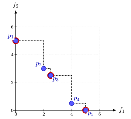
Figure 2: Points on a Pareto front approximation form an ordered l1 ‘staircase’: The red points form the most diverse 3-point subset.

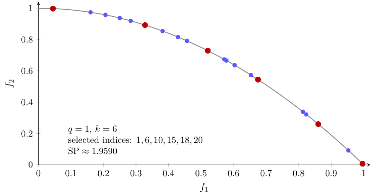
Figure 3: Subset selection of 6 points maximizing the Solow–Polasky diversity on a 2-D Pareto front approximation.

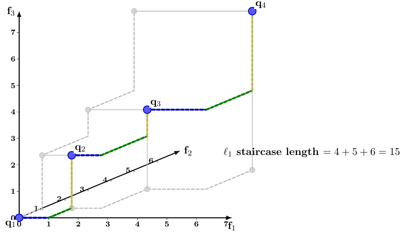
Figure 4: A staircase in three dimensions. The lengths of the connecting right-angle paths are the Manhattan or l1 distances between points. Beyond nearest neighbors additivity can be used to compute l1 distance.