Exact Hypervolume Subset Selection in 3-D: Implementing a Galactic Algorithm

Michael T. M. Emmerich, University of Jyväskylä, Finland, September 2026

In 2017 Karl Bringmann, Sergio Cabello and I showed that selecting the best ${k}$ out of ${n}$ points with respect to the hypervolume indicator is NP-hard already in three dimensions, that it can nevertheless be solved in time ${n^{O(\sqrt{k})}}$ , and that it admits an efficient polynomial-time approximation scheme (EPTAS) in every fixed dimension [BCE2017]. Both algorithms were described on paper only. This note reports on a complete implementation in Python with Numba-compiled kernels [LPS2015], on what it takes to make the constructions executable, and on an honest answer to the question every practitioner asks first: does it beat brute force? Code, tests, experiment scripts and an 11-page technical report are available at github.com/emmerichmtm/HSSP-3D [E2026].

Paper: K. Bringmann, S. Cabello, M. T. M. Emmerich, Maximum Volume Subset Selection for Anchored Boxes, SoCG 2017, LIPIcs 77, 22:1–22:15; full version arXiv:1803.00849.

Code: https://github.com/emmerichmtm/HSSP-3D (Python + Numba; source code MIT, report and data CC BY 4.0).

Technical report: report/report.pdf in the repository.

1. The problem

A point ${p \in \mathbb{R}^3_{>0}}$ spans the anchored box ${\mathrm{box}(p) = [0,p_1]\times[0,p_2]\times[0,p_3]}$ . For a finite point set ${Q}$ let ${\mathcal{U}(Q)}$ be the union of its boxes and ${\mu(Q) = \mathrm{vol}(\mathcal{U}(Q))}$ . Given ${n}$ points ${P}$ and a number ${k}$ , volume selection asks for

$\displaystyle {\mathrm{VolSel}(P,k) \;=\; \max_{S \subseteq P,\; |S| = k} \mu(S)}$

together with a maximizing subset. In multiobjective optimization this is the hypervolume subset selection problem (HSSP): for objective vectors ${f}$ that are to be minimized and a reference point ${r}$ , the substitution ${p = r - f}$ turns the hypervolume indicator [ZT1998] into ${\mu}$ . The problem appears whenever a large Pareto front approximation has to be represented by a few points, in bounded archives, and in the selection step of indicator-based algorithms such as SMS-EMOA [BNE2007].

What was known: in two dimensions the problem is polynomial, by dynamic programming along the front [ABBZ2009, BFK2014, KFPRDF2016]. For three and more dimensions the practical state of the art is the submodular greedy approach. The hypervolume indicator is a monotone submodular set function, so that repeatedly adding the point with the largest hypervolume contribution yields a ${(1-1/e)}$ -approximation in any dimension [NWF1978]. Guerreiro, Fonseca and Paquete [GFP2016] turned this observation into efficient algorithms for the HSSP: their greedy algorithms run in ${O(n(k+\log n))}$ time in two and in three dimensions, which matches the complexity of the exact two-dimensional algorithms. Their paper is the natural baseline for everything below, and the plain greedy algorithm serves as the reference heuristic in all experiments of this note. All exact algorithms for three and more dimensions enumerate, explicitly or implicitly, all ${\binom{n}{k}}$ subsets, each of which can be evaluated in ${O(k \log k)}$ time in three dimensions [BFLPV2009].

2. The exact algorithm in a nutshell

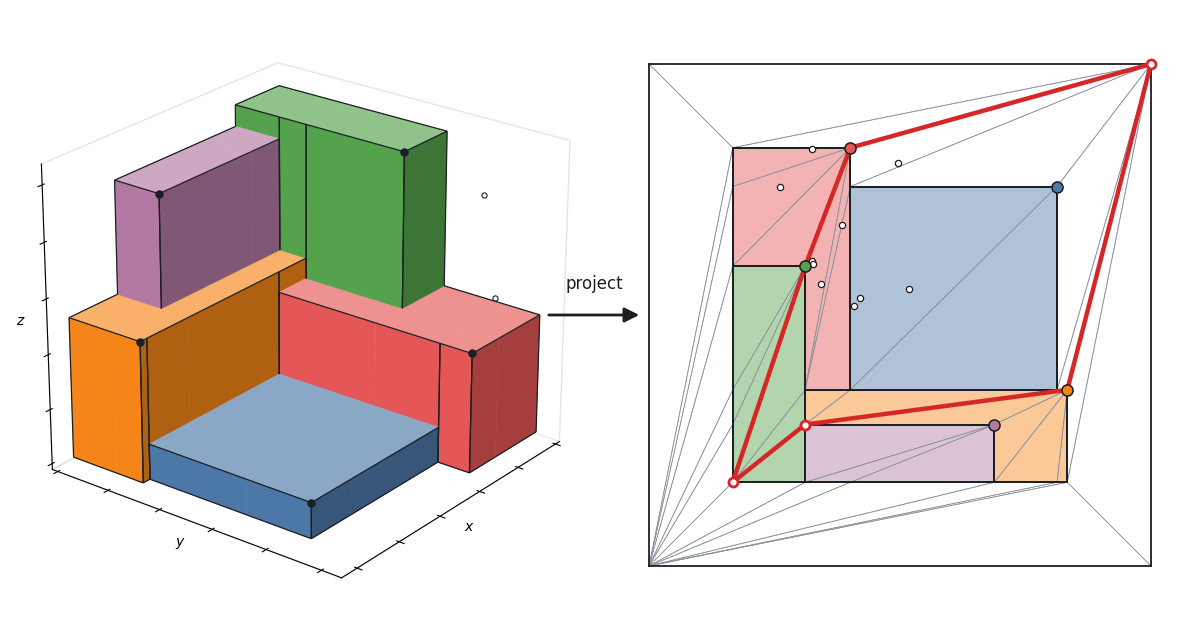
The key observation of [BCE2017] is that the boundary of ${\mathcal{U}(Q)}$ , projected onto the ${xy}$ -plane, is a planar graph with ${O(|Q|)}$ vertices: corners ${v_q}$ of the boxes, T-junctions where the boundary of one box disappears behind another, and vertices on the axes. Each bounded face ${f(q,Q)}$ is the region in which ${q}$ is the highest box. After a canonical triangulation (fans inside every face, and the outer face triangulated towards the corners of an enclosing square ${\sigma}$ ) one obtains a triangulation ${T(Q)}$ of ${\sigma}$ .

Planar graphs have small balanced separators. By Miller’s theorem [Miller1986], the triangulation ${T(Q^*)}$ of an optimal solution contains a simple cycle ${\gamma}$ with ${O(\sqrt{k})}$ vertices such that at most ${2k/3}$ of the corners ${v_q}$ lie on either side. The cycle is defined by only ${O(\sqrt{k})}$ points ${P_\gamma}$ of the solution. The algorithm therefore guesses these points and the cycle, which costs ${n^{O(\sqrt{k})}}$ trials, cuts the plane along ${\gamma}$ , and recurses on both sides with budgets of at most ${2k/3}$ .

Making the two sides independent is the delicate part, since a box chosen on one side also covers volume on the other. The paper resolves this with subproblems ${(S, D, \ell)}$ : a set ${S}$ of points that are already fixed, a polygonal domain ${D}$ whose boundary consists of edges of ${T(S)}$ (the domain is called ${S}$ -compliant), and a budget ${\ell}$ of points that may still be chosen inside the cylinder ${D \times \mathbb{R}}$ . Two values are attached to a subproblem,

$\displaystyle {\Phi_{\mathrm{free}}(S,D,\ell) \;=\; \max \{ \mathrm{vol}(\mathcal{U}(S\cup Q) \cap (D\times\mathbb{R})) \;:\; Q \subseteq P\cap(D\times\mathbb{R}),\ |Q| \le \ell \},}$

and ${\Phi_{\mathrm{comp}}(S,D,\ell)}$ , the same maximum restricted to those ${Q}$ for which ${D}$ is also ${(S\cup Q)}$ -compliant. The dynamic programme evaluates

$\displaystyle {\Psi(S,D,\ell) \;=\; \max_{\pi}\ \sum_{(S^{\prime},D_i,\ell_i)\in\pi} \Psi(S^{\prime},D_i,\ell_i),}$

where ${\pi}$ ranges over the valid partitions: a set ${S_0}$ of ${O(\sqrt{|S|+\ell})}$ further points, ${S^{\prime} = S\cup S_0}$ , a subdivision of ${D}$ into ${S^{\prime}}$ -compliant domains ${D_i}$ , and budgets ${\ell_i \le 2\ell/3}$ with ${|S_0| + \sum_i \ell_i = \ell}$ . Small budgets, ${\ell = O(\sqrt{k})}$ , are solved by enumeration. The correctness proof is a sandwich,

$\displaystyle {\Phi_{\mathrm{comp}}(S,D,\ell) \;\le\; \Psi(S,D,\ell) \;\le\; \Phi_{\mathrm{free}}(S,D,\ell),}$

and at the root both bounds coincide with ${\mathrm{VolSel}(P,k)}$ . The upper bound holds because every valid partition glues feasible solutions into a feasible solution. The lower bound holds because the separator of the optimal solution is among the partitions that are tried. Along every chain of the recursion ${|S| = O(\sqrt{k})}$ , which bounds the number of subproblems and the work per subproblem by ${n^{O(\sqrt{k})}}$ .

3. What it takes to make this executable

A common vertex space. Compliance compares edges of different triangulations. Every vertex of every ${T(Q)}$ has the ${x}$ -coordinate of some input point (or of an axis, or of a side of ${\sigma}$ ), and likewise for ${y}$ . Identifying vertices by their pair of coordinate ranks gives global integer vertex identifiers, so that edges and triangles of all triangulations are directly comparable and the defining points ${P_v}$ of a vertex can be read off its identifier.

The triangulation. Points are processed by decreasing ${z}$ ; the staircase of each face is traced through the two-dimensional skyline of the higher boxes, in ${O(|Q|^2)}$ time. Inside a triangle the height of the union is constant, hence for a compliant domain

$\displaystyle {\mathrm{vol}(\mathcal{U}(Q)\cap(D\times\mathbb{R})) \;=\; \sum_{t \in T(Q),\ t\subseteq D} \mathrm{area}(t)\cdot z_{\mathrm{owner}(t)} .}$

No clipping of boxes against polygons is ever needed. The unit tests check, for all subsets of several point sets, Euler’s formula ( ${2|V|-6}$ triangles), conformity, the total area, and equality of this sum for ${D=\sigma}$ with an independently computed exact hypervolume.

Compliance in linear time. A domain is handed to another triangulation as its list of directed boundary edges. A stamped edge table tells whether all of them are present (this is compliance), and a flood fill from the triangles to their left collects the triangles inside ${D}$ .

Partitions from cycles. For every candidate ${S_0}$ all simple cycles ${\gamma}$ of ${T(S\cup S_0)}$ of bounded length with ${P_\gamma \setminus S = S_0}$ that cut ${D}$ are enumerated by depth-first search; each cycle is generated once, from its lowest-ranked edge interior to ${D}$ , with pruning by breadth-first distance and by the number of points still to be covered. Cycles inducing the same subdivision are merged, and the budgets of the components are optimized by a max-plus knapsack over memoized subproblems.

The constants are parameters. The ${O(\cdot)}$ -notation hides three constants: the base-case threshold ${\lceil c_b\sqrt{k}\,\rceil}$ , the cycle length ${\lceil c_\gamma\sqrt{|S|+\ell}\,\rceil}$ and the separator size ${\lceil c_s\sqrt{|S|+\ell}\,\rceil}$ . For any fixed values the running time is ${n^{O(\sqrt{k})}}$ and the output is a feasible set, hence a lower bound. Optimality is proven only for the constants of Miller’s theorem: ${T(Q)}$ has at most ${5|Q|+5}$ vertices and a quadrilateral outer face, which gives ${|\gamma| \le 4\sqrt{5(|S|+\ell)+5}}$ and ${|P_\gamma|\le 2|\gamma|}$ . With these values the bound on ${|S_0|}$ drops below ${|S|+\ell}$ only beyond 320 points, so for every instance that can be run the proven algorithm degenerates into enumeration. The experiments therefore use ${c_b = 1}$ , ${c_\gamma = 2.5}$ , ${c_s = 1}$ , for which the separator recursion is really exercised, and compare with brute force.

4. Does it compute the optimum?

Yes, on everything that could be checked. On random samples of the DTLZ1 and DTLZ2 Pareto fronts [DTLZ2005] with ${n=15}$ and ${k\in\{3,4,5\}}$ , the dynamic programme returned the brute-force optimum, in fact the identical subset, in 36 of 36 runs, both with all valid partitions and with cycle separators only. The plain greedy algorithm was sub-optimal on 13 of the 18 instances, so the agreement is not inherited from a greedy incumbent. With the base case lowered to a single point, which forces nested separators and proper sub-polygons as domains, 12 of 12 runs with ${n=10}$ were optimal. When the constants are made too small (only one new point allowed on a separator) no balanced compliant separator exists; the recursion then places ${k-1}$ points, the last one is added greedily, and the result is merely a lower bound (4 of 6 optimal, gap up to 0.54 percent). From two points on a separator onwards, all instances were solved optimally.

5. Does it beat brute force?

No, not on any instance that can be run, and it is worth understanding why. For ${n=15}$ and ${k=5}$ brute force needs about a millisecond for its 3003 subsets, the dynamic programme between 27 and 58 seconds; a run with ${k=6}$ was stopped after 90 minutes. Even on the most favourable family I could construct (chain-like instances that possess a balanced separator through two points at every level, solved with the smallest constants that work) ${n=16}$ , ${k=6}$ did not finish within ten minutes. The reason is simple: ${\binom{n}{k}\le 2^n}$ , so for small ${n}$ enumeration is never expensive, whatever ${k}$ . The square root in the exponent pays off only when ${n \gg k \gg 1}$ .

To locate the cross-over I bounded the number of elementary operations of the implementation from above (choices of ${S_0}$ , of the cycle, of a component and of a budget at every level, plus the base cases) and compared it with the exact cost ${\binom{n}{k}k^2}$ of enumeration:

${n}$	${k}$	separator DP (upper bound)	brute force	fewer operations
${\le 10^3}$	any			brute force
${10^6}$	50	${10^{315}}$	${10^{239}}$	brute force
${10^6}$	79	${10^{360}}$	${10^{361}}$	DP (cross-over)
${10^6}$	200	${10^{656}}$	${10^{830}}$	DP, by a factor ${10^{174}}$
${10^6}$	1000	${10^{1433}}$	${10^{3438}}$	DP, by a factor ${10^{2005}}$

With the proven constants there is no cross-over at all for ${n\le 10^9}$ and ${k\le 3000}$ . The advantage of the algorithm is real, and it grows without bound, but it lives entirely in a regime in which neither method can be executed.

What is a galactic algorithm? Algorithms of this kind have a name. In a post on the blog Gödel’s Lost Letter and P=NP, Richard Lipton called an algorithm galactic if its asymptotic behaviour is wonderful but it is never used to compute anything, at least not on “terrestrial data sets” [L2010, LR2013]; the concept is Lipton’s, the name was coined by Ken Regan. The term is descriptive, not dismissive. Asymptotic analysis allows us to predict the running time of an algorithm without ever executing it, and sometimes the prediction is that the algorithm wins only for inputs of astronomical size, or that a less sophisticated method outperforms it on all realistic data. Lipton lists Shor’s quantum factoring algorithm (for the time being) and the polynomial-time algorithms that follow from the Robertson–Seymour graph minor theorem among his examples; fast matrix multiplication with exponent below 2.38 is another one that is often quoted. According to Lipton such algorithms nevertheless earn their place: they may contain techniques that lead to usable algorithms, they may become practical when computer architectures change, they may start a series of improvements that ends in a practical method, and they may show that a conjectured lower bound is wrong.

The ${n^{O(\sqrt{k})}}$ algorithm is galactic in exactly this sense. Its value is structural: it tells us that the exponent ${k}$ , which all earlier exact algorithms have, is not necessary (the last of the four roles above), and the implementation shows that the compliance-based recursion is correct as stated and yields tested building blocks (the triangulation, compliant domains, cycle-induced partitions) for more practical separator-based methods.

6. The approximation scheme

The EPTAS of [BCE2017] adapts the shifting technique of Hochbaum and Maass [HM1985] to anchored boxes. All boxes intersect near the origin, so the input cannot be broken into independent pieces; the remedy is an exponential grid, that is, a regular grid in a log-log plot. For ${d=3}$ let

$\displaystyle {\beta = (1-\varepsilon)^{-1/d}, \qquad \tau = \lfloor d/\varepsilon \rfloor + 1,}$

and let ${\lambda = \beta^{g}}$ be the smallest power of ${\beta}$ that is larger than ${d/\varepsilon}$ .

The positive orthant is divided into regions ${\prod_i [\lambda^{x_i},\lambda^{x_i+1})}$ . For each of the ${\tau^d}$ offsets ${\bar\ell}$ , the regions with ${x_i \equiv \ell_i \pmod{\tau}}$ for some ${i}$ form thick grid boundaries. The scheme deletes the points in the boundaries, partitions the remaining points into grid cells, rounds all coordinates down to powers of ${\beta}$ , solves every cell exactly for all budgets, distributes the budget ${k}$ over the cells by dynamic programming, and returns the best offset. Shifting, rounding and treating the cells as independent each lose a factor ${1-\varepsilon}$ . With ${V}$ the value of the best offset and ${S}$ the returned set of original points,

$\displaystyle {\mu(S) \;\ge\; (1-\varepsilon)\,V \qquad \text{and} \qquad V \;\ge\; (1-\varepsilon)^2\, \mathrm{VolSel}(P,k),}$

and hence

$\displaystyle {\mu(S) \;\ge\; (1-\varepsilon)^3\, \mathrm{VolSel}(P,k).}$

The second inequality has a practical consequence that is easy to overlook: ${V/(1-\varepsilon)^2}$ is a certified upper bound on the unknown optimum. The implementation returns it together with the solution, and it certifies any other solution as well, for instance the greedy one. Internally, points are represented by integer exponents ${e_i = \lfloor \log_\beta p_i \rfloor}$ , so that regions, cells and rounded points are exact integer quantities; rounded points dominated within their cell are dropped, and the solution of a cell is cached, because the same group of points forms a cell for many offsets.

Against the optimum ( ${n=15}$ , ${k=5}$ ; DTLZ1, DTLZ2 and instances whose coordinates span 20 orders of magnitude; 45 runs) the guarantee and the upper bound held everywhere, as they must. The observed ratios ${\mu(S)/\mathrm{OPT}}$ are far better than the worst case:

${\varepsilon}$	guaranteed ${(1-\varepsilon)^3}$	worst observed ratio	certified ratio ${\mu(S)/\mathrm{UB}}$	offsets ${\tau^3}$
0.5	0.125	0.927	about 0.32	343
0.25	0.422	0.979	about 0.64	2197
0.1	0.729	0.994	about 0.85	29791

For ${\varepsilon\le 0.25}$ the worst ratio of the scheme on the DTLZ instances is better than that of greedy (0.961 on DTLZ1, 0.976 on DTLZ2).

Beyond enumeration. On instances ${p = 10^{u}}$ with ${u}$ spread over a plane ${u_1+u_2+u_3 = c}$ and ${|u_i|\le 40}$ , that is, coordinates over 80 orders of magnitude and boxes of comparable volume, the grid splits the input into roughly 50 to 190 sparsely populated cells. With ${n=100}$ to ${400}$ points and ${k=10}$ to ${20}$ the scheme needs between 0.1 seconds and a few minutes, whereas brute force would have to enumerate up to ${10^{33}}$ subsets. This is a measured advantage over enumeration. Two caveats belong to an honest account. First, the submodular greedy algorithm [GFP2016] is faster still (a few milliseconds even in my naive implementation, which recomputes hypervolumes instead of updating contributions as in [GFP2016]) and its solutions are 0.2 to 3.6 percent better on these instances; widely spread boxes overlap little, which makes the instances easy. Second, the a-priori guarantee is weak for those ${\varepsilon}$ for which cells remain enumerable. What the scheme adds in practice is the certificate: for ${\varepsilon = 0.25}$ it proves that the returned set, and therefore also the better greedy set, is within a factor of about 0.65 of the optimum, slightly more than the ${1-1/e\approx 0.632}$ that is known for greedy a priori.

The exponential term ${2^{O((\varepsilon^{-2}\log(1/\varepsilon))^d)}}$ of the running time is the enumeration inside a cell. A cell spans 5.6, 14 and 46 orders of magnitude per coordinate for ${\varepsilon = 0.5}$ , ${0.25}$ and ${0.1}$ . For a typical Pareto front approximation all points therefore share a single cell, and the scheme reduces to deleting boundary points, rounding and enumeration; the implementation refuses to run rather than to enumerate more than ${5\cdot 10^7}$ subsets of one cell.

7. Take-aways and open questions

(1) Both algorithms of [BCE2017] are correct as stated and can be implemented faithfully; all deviations (parameterized constants, cycle-generated partitions, exact budgets, optional branch and bound) are documented in the report and do not affect correctness or the running-time bound.

(2) The ${n^{O(\sqrt{k})}}$ bound is a statement about the structure of the problem, not a recipe for a solver. In three dimensions and for practical sizes, enumeration, greedy [GFP2016] and integer programming remain the methods of choice.

(3) The certified upper bound of the EPTAS is a useful by-product. A tighter, cheaper certificate for HSSP solutions in three dimensions would be valuable in benchmarking.

(4) Open since 2017: is there a matching lower bound ${n^{\Omega(\sqrt{k})}}$ under the Exponential Time Hypothesis for ${d=3}$ , and ${n^{\Omega(k)}}$ for ${d\ge 4}$ ? Or is there a faster algorithm, say with exponent ${O(k^{1-1/d})}$ ? And do the constants of the separator approach improve for Pareto fronts with additional structure, such as the staircases of the projection graph?

8. Code and reuse

pip install -e . # repository: https://github.com/emmerichmtm/HSSP-3D

from hssp3d import solve, solve_eptas, solve_brute_force, dtlz2_front

F = dtlz2_front(15, seed=0) # minimization objective vectors

exact = solve(F, k=5, reference=[1.1, 1.1, 1.1]) # separator dynamic programme

approx = solve_eptas(F, k=5, eps=0.25, reference=[1.1, 1.1, 1.1])

print(exact.subset, exact.hypervolume)

print(approx.hypervolume, approx.stats["upper_bound"], approx.stats["certified_ratio"])

The report, documentation and result data are licensed under CC BY 4.0, the source code under the MIT License. Please cite this note as: M. T. M. Emmerich, A Galactic Algorithm Implementation: Hypervolume Subset Selection in 3-D, MODA News, emmerix.net, September 19, 2026.

References

[ABBZ2009] A. Auger, J. Bader, D. Brockhoff, E. Zitzler. Investigating and exploiting the bias of the weighted hypervolume to articulate user preferences. In Proc. Genetic and Evolutionary Computation Conference (GECCO), pp. 563–570. ACM, 2009.

[BCE2017] K. Bringmann, S. Cabello, M. T. M. Emmerich. Maximum volume subset selection for anchored boxes. In 33rd International Symposium on Computational Geometry (SoCG 2017), LIPIcs 77, pp. 22:1–22:15, 2017. Full version: arXiv:1803.00849.

[BFK2014] K. Bringmann, T. Friedrich, P. Klitzke. Two-dimensional subset selection for hypervolume and epsilon-indicator. In Proc. Genetic and Evolutionary Computation Conference (GECCO), pp. 589–596. ACM, 2014.

[BFLPV2009] N. Beume, C. M. Fonseca, M. López-Ibáñez, L. Paquete, J. Vahrenhold. On the complexity of computing the hypervolume indicator. IEEE Transactions on Evolutionary Computation 13(5):1075–1082, 2009.

[BNE2007] N. Beume, B. Naujoks, M. Emmerich. SMS-EMOA: Multiobjective selection based on dominated hypervolume. European Journal of Operational Research 181(3):1653–1669, 2007.

[DTLZ2005] K. Deb, L. Thiele, M. Laumanns, E. Zitzler. Scalable test problems for evolutionary multiobjective optimization. In Evolutionary Multiobjective Optimization, pp. 105–145. Springer, 2005.

[E2026] M. T. M. Emmerich. An implementation of the n^O(sqrt k) algorithm and of the EPTAS for 3-D hypervolume subset selection. Technical report and software, University of Jyväskylä, 2026. https://github.com/emmerichmtm/HSSP-3D.

[GFP2016] A. P. Guerreiro, C. M. Fonseca, L. Paquete. Greedy hypervolume subset selection in low dimensions. Evolutionary Computation 24(3):521–544, 2016. doi:10.1162/EVCO_a_00188.

[HM1985] D. S. Hochbaum, W. Maass. Approximation schemes for covering and packing problems in image processing and VLSI. Journal of the ACM 32(1):130–136, 1985.

[KFPRDF2016] T. Kuhn, C. M. Fonseca, L. Paquete, S. Ruzika, M. M. Duarte, J. R. Figueira. Hypervolume subset selection in two dimensions: Formulations and algorithms. Evolutionary Computation 24(3):411–425, 2016.

[L2010] R. J. Lipton. Galactic algorithms. Gödel’s Lost Letter and P=NP (blog), October 23, 2010. https://rjlipton.com/2010/10/23/galactic-algorithms/.

[LPS2015] S. K. Lam, A. Pitrou, S. Seibert. Numba: a LLVM-based Python JIT compiler. In Proc. 2nd Workshop on the LLVM Compiler Infrastructure in HPC. ACM, 2015.

[LR2013] R. J. Lipton, K. W. Regan. People, Problems, and Proofs, chapter “David Johnson: Galactic Algorithms”. Springer, 2013.

[Miller1986] G. L. Miller. Finding small simple cycle separators for 2-connected planar graphs. Journal of Computer and System Sciences 32(3):265–279, 1986.

[NWF1978] G. L. Nemhauser, L. A. Wolsey, M. L. Fisher. An analysis of approximations for maximizing submodular set functions – I. Mathematical Programming 14(1):265–294, 1978.

[ZT1998] E. Zitzler, L. Thiele. Multiobjective optimization using evolutionary algorithms – a comparative case study. In Parallel Problem Solving from Nature (PPSN V), LNCS 1498, pp. 292–301. Springer, 1998.