Isolating Noise from Signal in the Prime Number Distribution

A Deep Dive into Riemann’s Hypothesis: Isolating Noise from Signal in the Prime Distribution

Date: 2026-02-14

Author: Michael Emmerich

The primes look orderly from far away and chaotic up close. At a large scale they follow clean laws: the density of primes near $x$ is about $1/\log x$ , and the prime-counting function $\pi(x)$ is well approximated by $\mathrm{li}(x)$ . But if you zoom in, the clean curve starts to wobble: the primes come a bit earlier, then a bit later, and the error term flips sign in a way that feels noisy.

Riemann’s 1859 insight was that this “noise” is not random at all. It is built from a superposition of oscillations whose frequencies come from the nontrivial zeros of the zeta function $\zeta(s)$ . The Riemann Hypothesis (RH), perhaps the most intriguing unsolved problem in mathematics, says that all those zeros have real part $\tfrac12$ . In this essay I focus on the oscillatory term: what it is, where it comes from historically, and how to see it in a small interactive visualization.

A supporting app (as usual for my blog entries) is available at https://trinket.io/library/trinkets/0d5924c81cfd. It displays three linked views: a circle in the complex plane traced by $20^{\sigma+it}$ , its image under a complex logarithmic-integral continuation, and a small plot that shows the per-zero oscillatory contributions.

Signal: the smooth main term

A simple “signal” in the prime distribution is the large-scale growth of $\pi(x)$ . One of the most successful smooth approximations is the logarithmic integral

$\displaystyle \mathrm{li}(x)=\text{p.v.}\int_0^x \frac{dt}{\log t},$

understood as a principal value at $t=1$ . At the level of intuition, $\mathrm{li}(x)$ captures that primes thin out slowly, on the scale of $\log x$ .

This clean approximation is the part you see when you squint.

Noise: the oscillatory correction from zeta zeros

The striking part is that the deviation from the smooth term can be expressed using the zeros of $\zeta(s)$ . Different explicit formulas exist (depending on whether one counts primes, prime powers, or uses weights), but their shared backbone can be summarized schematically as:

$\displaystyle \text{(prime-counting)}\;\approx\; \mathrm{li}(x)\;-\;\sum_{\rho}\mathrm{li}(x^{\rho})\;+\;\text{(smaller correction terms)}. \qquad (1)\;$

Here $\rho$ runs over the nontrivial zeros of $\zeta(s)$ . The first term is the “signal,” and the sum over zeros supplies the “noise” – not random noise, but a structured oscillatory interference pattern.

Why oscillatory? Because a typical zero can be written as

$\displaystyle \rho=\beta+i\gamma, \qquad (2)\;$

and for real $x>1$ ,

$\displaystyle x^\rho = x^{\beta+i\gamma} = x^\beta e^{i\gamma\log x}. \qquad (3)\;$

The factor $e^{i\gamma\log x}$ is a pure rotation. So each zero contributes a wave with frequency $\gamma$ in the variable $\log x$ , and the sum over many zeros is a superposition of many such waves.

This is the historical source of the language “periodic term” in older accounts: the oscillations are not literally periodic in $x$ , but they are strongly oscillatory in $\log x$ .

A short historical detour

Riemann’s 1859 memoir connected primes to $\zeta(s)$ in a way that was startlingly ahead of its time. The explicit formulas that make the schematic relationship in (1) precise were clarified and developed further by later mathematicians, notably von Mangoldt, who explained how the sum over zeros appears and how additional correction terms enter. Over the 20th century, these formulas became a workhorse: knowledge about zeros translates into quantitative statements about the irregularities in prime distribution.

In that sense, RH is not merely a statement about where zeros sit in the complex plane. It is a statement about how big the prime “noise” can get.

Why the conjugate symmetry does not cancel the oscillation

A common first reaction is: zeros come in conjugate pairs, so do they cancel?

They do not. Conjugate pairing turns complex oscillations into real oscillations.

If $\rho=\beta+i\gamma$ is a zero, then $\overline{\rho}=\beta-i\gamma$ is also a zero. For real $x>1$ ,

$\displaystyle x^{\overline{\rho}}=\overline{x^\rho}. \qquad (4)\;$

With branch choices compatible with conjugation (the natural setting for real $x$ ),

$\displaystyle \mathrm{li}(x^{\overline{\rho}})=\overline{\mathrm{li}(x^\rho)}. \qquad (5)\;$

Hence

$\displaystyle \mathrm{li}(x^\rho)+\mathrm{li}(x^{\overline{\rho}})=2\Re\!\big(\mathrm{li}(x^\rho)\big). \qquad (6)\;$

So the imaginary parts cancel, but the real part doubles. This is exactly the same mechanism as

$\displaystyle e^{i\theta}+e^{-i\theta}=2\cos\theta. \qquad (7)\;$

The oscillation survives – now as a real cosine-like term.

Why the critical line matters

RH says $\beta=\tfrac12$ for every nontrivial zero $\rho=\beta+i\gamma$ . In the expression $x^\rho=x^\beta e^{i\gamma\log x}$ , the exponent $\beta$ controls the amplitude scale. If $\beta$ were larger, the oscillatory correction would be larger; if smaller, it would be smaller. Under RH, the amplitude behaves like $x^{1/2}$ (up to additional factors depending on the chosen explicit formula and on $\gamma$ ).

This is why RH is often described as a sharp statement about the size of the error term in prime counting: it puts the oscillations under tight control.

The three-panel view in the visualization

The supporting app is designed as a small “oscillation microscope.” It does not compute $\pi(x)$ . Instead it isolates the building block

$\displaystyle \mathrm{Li}\!\left(20^{\sigma+it}\right)\quad\text{and highlights the special parameter values } t=\pm\gamma_k. \qquad (8)\;$

where $\tfrac12+i\gamma_k$ are the first nontrivial zeros of $\zeta(s)$ .

Panel 1 (top-left): tracing a circle

For a real base $B>0$ and real $\sigma$ ,

$\displaystyle z(t)=B^{\sigma+it}=\exp\!\big((\sigma+it)\ln B\big)=B^\sigma e^{it\ln B}. \qquad (9)\;$

So $|z(t)|=B^\sigma$ is constant in $t$ and the curve is an exact circle centered at the origin. The marked points at $t=\pm\gamma_k$ are mirror images because $z(-t)=\overline{z(t)}$ .

Panel 2 (right): a smooth complex continuation of Li

On the right, the app draws a complex logarithmic-integral continuation along the same parameter values. A practical way to produce a continuous curve along $t$ is to write it using the exponential integral:

$\displaystyle w(t)=\mathrm{Ei}\!\big((\sigma+it)\ln B\big). \qquad (10)\;$

which follows the parameter smoothly (avoiding branch-cut jumps that can occur if one forces a principal logarithm on a looping path). The marked points again come in conjugate pairs: $w(-\gamma_k)=\overline{w(\gamma_k)}$ .

Plot below the circle: per-zero oscillatory contributions

The bottom plot connects directly to the “conjugate pairing yields a real oscillation” idea. For each $k$ it computes

$\displaystyle C_k \;=\; w(\gamma_k)+w(-\gamma_k)\;=\;2\Re\!\big(w(\gamma_k)\big). \qquad (11)\;$

and displays $C_k$ as a stem plot against the zero index $k$ . In other words, you can see that the pair does not cancel: it produces a real contribution that can be positive or negative.

A small pause on the critical line

The app wiggles $\sigma$ slightly around $\tfrac12$ . Whenever it hits the critical line $\sigma=\tfrac12$ exactly, it pauses for a second and shows the marked points in green. This is not a computational claim about RH; it is a visual cue to compare the geometry “on the line” and “near the line.” It is an invitation to treat $\sigma=\tfrac12$ as the place where the oscillatory story is meant to be read.

Closing thought

If you like, you can interpret the signal-plus-noise idea in (1) as:

$\displaystyle \mathrm{li}(x)\quad\text{(signal)} \qquad + \qquad \left(-\sum_\rho \mathrm{li}(x^\rho)\right)\quad\text{(structured noise)}. \qquad (12)\;$

The “noise” is not random; it is made from frequencies $\gamma_k$ . Riemann’s hypothesis then becomes a very precise claim about the amplitude of this noise: every contributing wave has the same amplitude scale $x^{1/2}$ , because every zero sits exactly on the critical line.

Further reading (optional)

B. Riemann. Über die Anzahl der Primzahlen unter einer gegebenen Grösse. Monatsberichte der Berliner Akademie, 1859.
H. M. Edwards. Riemann’s Zeta Function. Dover, 2001.
A. Ivić. The Riemann Zeta-Function: Theory and Applications. Dover, 2003.

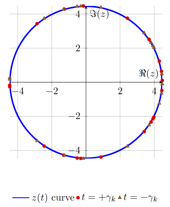
Figure 1: ${20^{0.5 + si}}$ , where $s=\rho_i$ are marked for the first 20 zeros Riemann’s Zeta function on the critical line.

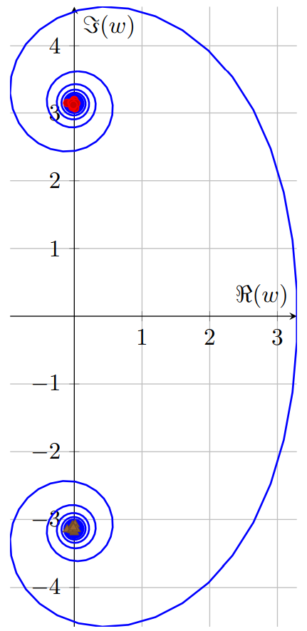
Figure 2: The function ${Li(20^{0.5+s i})}$ for different values of s with zeros of the Riemann Zeta function marked. The oscillations of the primes are the sums of the real part fluctuations of the zeros.

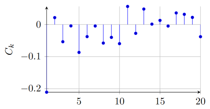
Figure 3: A paired component of the sum that makes up the periodic term in Riemann’s summation. It combines a zero with its conjugate zero. The values ${C_k}$ are the sum of the (equal) real parts at a zero where the real parts are defined as ${\Re(Li(20^{0.5+s i}))}$ .

Isolating Noise from Signal in the Prime Number Distribution

Share this:

Leave a comment Cancel reply