A very, very simple method to estimate Pi

Date: 2026-03-15

Author: Michael T.M. Emmerich

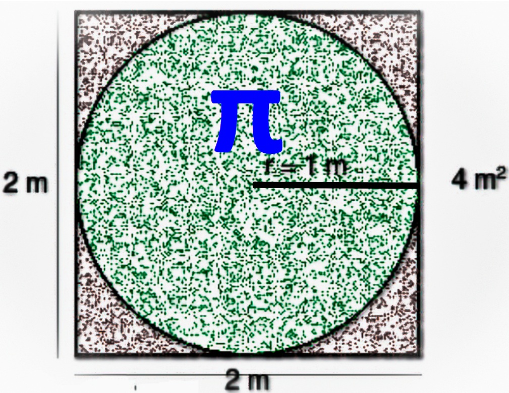
Every year, on March 14, mathematicians celebrate Pi Day. For my Mathematical Playground blog, I wished to post a short essay on a very, very simple Monte Carlo method for estimating $\pi$ . The nice aspect of this method is that it requires only a few lines of code, does not require irrational numbers in the computations, and rests on a very simple intuition. Mathematically, however, the estimation of the uncertainty of this approximation is even more interesting, and the same idea can also be applied to other Monte Carlo estimation methods. As the name Monte Carlo already suggests – Monaco being the town of casinos – randomness plays an essential role. My playground example could also serve as a small exercise for practicing basic concepts in probability theory and statistics.

The setup is easy to picture: take the unit circle, meaning a circle of radius $1\,\mathrm{m}$ , center it at the origin, and place it inside the square $[-1,1]\times[-1,1]$ . The square has side length $2$ , so its area is $4$ . The circle has area $\pi$ .

Now throw random points uniformly into the square and count how many land inside the circle. That is the whole idea.

The lovely part is that the computation itself does not use $\pi$ at all. We only test whether a sampled point is close enough to the center. That is all.

To make the idea concrete, I also wrote a small interactive Python simulation with an approximate 95% uncertainty band:

Interactive Monte Carlo Pi simulation

A very, very simple geometric idea

The circle has radius $1\,\mathrm{m}$ , so its area is exactly

$\displaystyle A = \pi \cdot 1^2 = \pi \,\mathrm{m}^2.$

The surrounding square is the set $[-1,1]\times[-1,1]$ , so its side length is $2\,\mathrm{m}$ and its area is

$\displaystyle 2\cdot 2 = 4\,\mathrm{m}^2.$

If we sample points uniformly in that square, then the fraction of points landing inside the circle estimates the fraction of the square covered by the circle. Since the square area is known, we can estimate the circle area by

$\displaystyle \widehat{A}_n = 4 \cdot \frac{\text{number of hits}}{n}.$

But the circle is the unit circle, so its area is exactly $\pi$ . Therefore

$\displaystyle \widehat{\pi}_n = \widehat{A}_n = 4\cdot\frac{\text{number of hits}}{n}.$

This keeps the method very direct: estimate the area of the unit circle, and you have estimated $\pi$ .

Why no knowledge of pi is needed

Suppose a sampled point has coordinates $(x,y)$ , where the origin is the center of the square and the circle. The point lies inside the unit circle exactly when its distance from the center is at most $1$ :

$\displaystyle \sqrt{x^2+y^2} \leq 1.$

Equivalently, and more conveniently for a computer, we check

$\displaystyle x^2+y^2 \leq 1.$

This is the whole algorithm. No trigonometry. No circumference formula. No prior knowledge of $\pi$ . Just random points and a distance test.

A tiny Python program

import random

n = 100000
hits = 0

for _ in range(n):
    x = 2 * random.random() - 1
    y = 2 * random.random() - 1
    if x*x + y*y <= 1:
        hits += 1

pi_est = 4 * hits / n
print(pi_est)

How to read the code

The two coordinates are sampled uniformly from $[-1,1]$ , so the point lies somewhere in the square of side length $2$ .
The condition x*x + y*y <= 1 checks whether the point is inside the unit circle.
The fraction of hits estimates how much of the square is covered by the circle.
Multiplying by the known square area $4$ gives the estimated circle area, which for the unit circle is also an estimate of $\pi$ .

An online moving-average version

If one wants to keep the simulation running as an anytime algorithm, there is a neat alternative that updates the estimate directly, without storing the total number of hits. For each sample, define

$\displaystyle Y_i = \begin{cases} 4, & \text{if point } i \text{ lands inside the circle,} \\ 0, & \text{otherwise.} \end{cases}$

Then $\widehat{\pi}_n$ is simply the average of the $Y_i$ . This means we can update the estimate by a moving-average formula:

$\displaystyle \widehat{\pi}_{n+1}=\widehat{\pi}_n+\frac{Y_{n+1}-\widehat{\pi}_n}{n+1}.$

In code, this looks as follows:

import random

pi_est = 0.0

for n in range(1, 100001):
    x = 2 * random.random() - 1
    y = 2 * random.random() - 1
    sample = 4.0 if x*x + y*y <= 1 else 0.0
    pi_est += (sample - pi_est) / n

print(pi_est)

This online form is mathematically equivalent to counting hits, but it is convenient when one wants to keep a running estimate forever. It uses constant memory and fits the spirit of an anytime algorithm: at every moment, the current value is the best estimate obtained so far.

Why this works

For each sampled point, define an indicator variable

$\displaystyle I_i = \begin{cases} 1, & \text{if point } i \text{ lands inside the circle,} \\ 0, & \text{otherwise.} \end{cases}$

Each $I_i$ is a Bernoulli random variable: either success or failure. After $n$ samples, the observed hit rate is

$\displaystyle \hat h_n = \frac{1}{n}\sum_{i=1}^n I_i.$

The estimator of the circle area is then

$\displaystyle \widehat{A}_n = 4\hat h_n,$

and because the unit circle has area $\pi$ , this is also the estimator of $\pi$ :

$\displaystyle \widehat{\pi}_n = 4\hat h_n.$

This is an example of a Monte Carlo method: a method that uses repeated random sampling to estimate an unknown quantity.

The non-trivial part: how accurate is the estimate?

The estimate itself is easy. The more interesting question is: how much should we trust it after $n$ samples?

This belongs to what is often called uncertainty quantification in statistics and computer science. The estimate alone is not the whole story. It is often important to report, in addition, how uncertain the estimate still is.

Let $h$ denote the true hit probability, that is, the probability that a uniformly sampled point from the square lands inside the unit circle. Then each $I_i$ is Bernoulli with parameter $h$ , so

$\displaystyle \mathrm{Var}(I_i)=h(1-h).$

The average hit rate $\hat h_n$ therefore has variance

$\displaystyle \mathrm{Var}(\hat h_n)=\frac{h(1-h)}{n}.$

Because $\widehat{\pi}_n = 4\hat h_n$ , the variance of the estimator of $\pi$ is

$\displaystyle \mathrm{Var}(\widehat{\pi}_n)=16\frac{h(1-h)}{n}.$

Hence the standard deviation is

$\displaystyle \mathrm{SD}(\widehat{\pi}_n)=4\sqrt{\frac{h(1-h)}{n}}.$

This formula already shows the key message: the uncertainty decreases only like $1/\sqrt{n}$ . So the method converges, but rather slowly.

A beginner-friendly estimated 95% band

Of course, the true hit probability $h$ is unknown. So in practice we replace it by the observed hit rate $\hat h_n$ and estimate the standard error by

$\displaystyle \widehat{\mathrm{SE}}(\widehat{\pi}_n)=4\sqrt{\frac{\hat h_n(1-\hat h_n)}{n}}.$

A common approximate 95% uncertainty interval is then

$\displaystyle \widehat{\pi}_n \pm 1.96\,\widehat{\mathrm{SE}}(\widehat{\pi}_n).$

Where does the $1.96$ come from? It comes from the standard normal, also called the Gaussian distribution. If $Z$ is standard normal, then

$\displaystyle \mathbb{P}(-1.96 \leq Z \leq 1.96)\approx 0.95.$

Equivalently,

$\displaystyle 1.96 \approx \Phi^{-1}(0.975),$

where $\Phi$ is the cumulative distribution function of the standard normal distribution. So yes – it comes from the inverse Gaussian distribution function, more precisely from the inverse cumulative distribution function.

This is the band shown in the interactive simulation. It gives the reader a sense not only of the estimate itself, but also of how noisy it still is after a given number of samples.

That extra layer – reporting uncertainty together with the estimate – is precisely what makes the simulation more than a toy. It introduces a central statistical idea in a very concrete setting.

Where this sits among methods for computing pi

Monte Carlo estimation is certainly not the fastest way to compute many digits of $\pi$ . There are far more efficient methods: classical polygon approximations going back to Archimedes, infinite series such as the Leibniz series and Machin-type formulas, arithmetic-geometric mean methods, Ramanujan-type series, and modern high-precision formulas such as the Chudnovsky series.

So why use Monte Carlo here at all? Because it is conceptually delightful. It connects geometry, probability, simulation, and statistics in one tiny experiment. It also teaches a lesson that is broader than $\pi$ : when we estimate something from data or randomness, we should often report both the estimate and its uncertainty.

References

Archimedes. (1897). The Works of Archimedes. Edited by T. L. Heath. Cambridge: Cambridge University Press.
Borwein, J. M., & Borwein, P. B. (1987). Pi and the AGM: A Study in Analytic Number Theory and Computational Complexity. New York: John Wiley & Sons.
Chudnovsky, D. V., & Chudnovsky, G. V. (1988). Approximation and complex multiplication according to Ramanujan. In Ramanujan Revisited (pp. 375-472). Boston: Academic Press.
Gentle, J. E. (2003). Random Number Generation and Monte Carlo Methods (2nd ed.). New York: Springer.
Hammersley, J. M., & Handscomb, D. C. (1964). Monte Carlo Methods. London: Methuen.
Rubinstein, R. Y., & Kroese, D. P. (2017). Simulation and the Monte Carlo Method (3rd ed.). Hoboken, NJ: John Wiley & Sons.

Try the interactive simulation

You can explore the app here:

https://trinket.io/library/trinkets/e2da81b48f3d

Watch the random points appear, see the running estimate move around, and observe how the 95% band gradually narrows. It is a very simple Pi Day experiment – but also a neat first encounter with uncertainty quantification.

A very, very simple method to estimate Pi

Share this:

Leave a comment Cancel reply