Nature doesn’t just have averages; it has extremes—the hottest day, the strongest wind, the largest daily rainfall, the highest flood. For extremes, a universal statistical law often appears: the Gumbel distribution. In this post, we meet it through a simple and realistic story about annual maximum rainfall, learn how a basic normalization makes its shape universal, and see how the constant 
A Natural Question: How Extreme Can the Weather Get?
Imagine a weather station recording the daily rainfall amounts 

Repeat for many years and you obtain a sequence of annual maxima 
Extreme Value Theory
Even if the daily rainfalls come from a wide class of “moderately tailed” distributions (exponential-like, gamma-like, even normal), the distribution of their maxima, after a simple normalization, tends to the same limiting shape:

which is the Gumbel distribution with location 


This is a cornerstone of Extreme Value Theory (EVT): it plays a role for maxima that’s analogous to the Central Limit Theorem for sums.
Euler–Mascheroni Constant Appears
In the standard Gumbel case (

![\mathbb{E}[X] \;=\; \gamma \approx 0.5772156649\ldots](https://s0.wp.com/latex.php?latex=%5Cmathbb%7BE%7D%5BX%5D+%5C%3B%3D%5C%3B+%5Cgamma+%5Capprox+0.5772156649%5Cldots&bg=ffffff&fg=000&s=0&c=20201002)
This is the same 
![\mathbb{E}[T_n] = n\ln n + \gamma n + \tfrac12 + o(1)](https://s0.wp.com/latex.php?latex=%5Cmathbb%7BE%7D%5BT_n%5D+%3D+n%5Cln+n+%2B+%5Cgamma+n+%2B+%5Ctfrac12+%2B+o%281%29&bg=ffffff&fg=000&s=0&c=20201002)
A Simple Rainfall Model
To see the Gumbel distribution in action, we can model each day’s rainfall as exponential with mean, say, 10 mm (many dry/small days, a few heavy ones). For each “year,” sample 365 daily values and record their maximum. Repeat across many years. The empirical histogram of these annual maxima fits a Gumbel curve remarkably well.
(I’ll add the Python code and plots as an appendix.)
The Simple Normalization Idea
The maxima get larger as we observe more samples. To compare maxima across different sample sizes (or across years and stations), we normalize them. Suppose we look at

There exist centering and scaling sequences 


converges in distribution to a standard Gumbel law:

Intuitively:
,
rescales the spread so the distribution doesn’t collapse to a spike.
After this shift-and-rescale, the histograms of different-sized maxima align to a stable shape (the Gumbel curve). Figure 1 illustrates this schematic “shift by
The Continuous Mirror
The Euler–Mascheroni constant


A beautiful continuous mirror of this discrete definition is


As we have seen, the same constant appears as the expected value of the Gumbel distribution:
![\displaystyle \mathbb{E}[X] = \int_{-\infty}^{\infty} x\, e^{-(x+e^{-x})}\,dx = \gamma.](https://s0.wp.com/latex.php?latex=%5Cdisplaystyle+%5Cmathbb%7BE%7D%5BX%5D+%3D+%5Cint_%7B-%5Cinfty%7D%5E%7B%5Cinfty%7D+x%5C%2C+e%5E%7B-%28x%2Be%5E%7B-x%7D%29%7D%5C%2Cdx+%3D+%5Cgamma.&bg=ffffff&fg=000&s=0&c=20201002)

Emil Julius Gumbel: The Man Behind the Curve
Emil Julius Gumbel (1891–1966) was a German mathematician, statistician, and outspoken pacifist. Emil Gumbel was a German mathematician, statistician, and passionate pacifist. Born in Munich, he studied under Felix Klein and worked on applying statistics to real-world hazards — floods, storms, and structural failures.
But Gumbel’s life took a dramatic turn: he openly opposed the rise of Nazism, publishing data on political murders and exposing right-wing violence in Germany. He was expelled from his academic post, fled to France, and later continued his career in the United States at Columbia University.
While in exile, Gumbel formalized the mathematics of extreme events, culminating in his book Statistics of Extremes (1958). His name now stands for one of the fundamental distributions in Extreme Value Theory—a field that underpins modern climate modeling, engineering safety, and risk management. Recently, the Gumbel distribution has even been applied in Bayesian multiobjective optimization and machine learning (Chugh & Evans, 2024).
Takeaways and DIY Projects
- Annual maxima of daily rainfall are naturally modeled by the Gumbel distribution.
- A simple normalization (shift by
- The Euler–Mascheroni constant
I have added two practical exercises with python code. In the first one you can experiment with a distribution (exponential) and by simulation experience yourself how the Gumbel distribution appears. The second example lets you experiment with real annual maximum rainfall data, which you can download from the internet for your city and check the fit to the Gumbel distribution, and check if there is a trend in the maxima.
References
- Emmerich, Michael (2024, October 11). Of Autumn Leaves and Coupon Collectors. Mathematical Playground. http://www.emmerix.net.
- Chugh, T., & Evans, A. (2024, March). Integrating Bayesian and evolutionary approaches for multi-objective optimisation. In International Conference on the Applications of Evolutionary Computation (Part of EvoStar) (pp. 391-406). Cham: Springer Nature Switzerland.
- E. J. Gumbel, Statistics of Extremes, Columbia University Press, 1958.
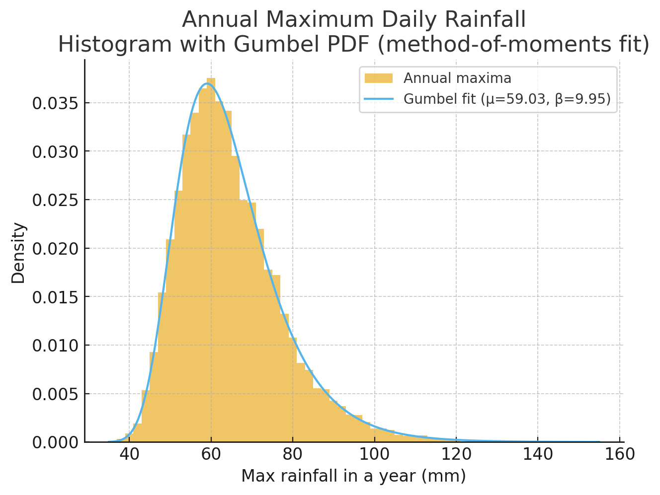
Figure 1. Example in Appendix 1. Normalization of maxima: raw maxima (left) shift and rescale to a stable Gumbel-shaped distribution (right). Arrows indicate “shift by
Appendix 1: Simulation of Gumbel distributed data set
Below is the Python code that produces the plot in Figure 1 for 20000 years and daily rainfall modeled as a exponential distribution:
- Simulates daily rainfall and records annual maxima across many years,
- Fits a Gumbel distribution to the maxima,
- Produces figures (histogram + fitted PDF).
What the script does (walkthrough)
-
Simulates daily rainfall
- Assumes Exponential(mean = 10 mm) for each day; 365 days per year.
- Runs for many years (
YEARS = 20000) to get a smooth distribution of annual maxima.
-
Computes annual maxima
- For each simulated year, takes the maximum daily rainfall. This yields a 1D array of yearly maxima.
-
Fits a Gumbel distribution via method of moments (no SciPy required)
- Uses the Gumbel facts:
-
Mean:
Variance: -
From the sample mean
and sample variance
:
![\mathbb{E}[X] = \mu + \gamma\,\beta](https://s0.wp.com/latex.php?latex=%5Cmathbb%7BE%7D%5BX%5D+%3D+%5Cmu+%2B+%5Cgamma%5C%2C%5Cbeta&bg=ffffff&fg=000&s=0&c=20201002)
![\mathrm{Var}[X] = \left(\pi^2/6\right)\beta^2](https://s0.wp.com/latex.php?latex=%5Cmathrm%7BVar%7D%5BX%5D+%3D+%5Cleft%28%5Cpi%5E2%2F6%5Cright%29%5Cbeta%5E2&bg=ffffff&fg=000&s=0&c=20201002)

"""
Histogram of Annual Maxima with Gumbel Fit (Method of Moments)

Overview
--------
This script simulates daily rainfall amounts for many years, computes the
annual maximum rainfall, and fits a Gumbel distribution to those maxima using
the method of moments (MoM). It then overlays the fitted Gumbel PDF on the
histogram of annual maxima and saves the figure as a PNG.

Why Gumbel?
-----------
The Gumbel distribution often appears as a limiting distribution for maxima
(e.g., yearly maximum daily rainfall), under broad conditions (Extreme Value
Theory).

Model Assumptions
-----------------
- Daily rainfall is modeled as Exponential(mean = 10 mm).
  This captures "many small, few large" rainfall days.
- 365 days per year.
- We simulate `YEARS` independent years to get a smooth histogram.

Gumbel(μ, β) Method-of-Moments
-------------------------------
For a random variable X ~ Gumbel(μ, β),
- E[X] = μ + γ β,  where γ is the Euler–Mascheroni constant
- Var[X] = (π^2 / 6) β^2
Thus, given sample mean m and sample variance s^2, the MoM estimators are:
- β̂ = sqrt(6 s^2) / π
- μ̂ = m − γ β̂

Outputs
-------
- PNG figure: 'gumbel_annual_max_hist_fit.png'
- The console prints fitted parameters μ̂ and β̂

Usage
-----
Run this file with Python 3. It requires only NumPy and Matplotlib.
"""

import numpy as np
import matplotlib.pyplot as plt

# ------------------- Configuration -------------------
SEED = 20251011
DAYS_PER_YEAR = 365
YEARS = 20000          # large for a smooth fit
DAILY_MEAN_MM = 10.0   # mean of exponential daily rainfall

# ------------------- Simulation ----------------------
rng = np.random.default_rng(SEED)

# Simulate daily rainfall: shape (YEARS, DAYS_PER_YEAR)
daily_rain = rng.exponential(DAILY_MEAN_MM, size=(YEARS, DAYS_PER_YEAR))

# Annual maxima: one maximum per simulated year
annual_max = daily_rain.max(axis=1)

# ------------------- Gumbel MoM fit ------------------
GAMMA = 0.5772156649015329

xbar = annual_max.mean()
s2 = annual_max.var(ddof=1)              # unbiased sample variance
beta_hat = np.sqrt(6.0 * s2) / np.pi     # β̂
mu_hat = xbar - GAMMA * beta_hat         # μ̂

print(f"Fitted Gumbel parameters (MoM): mu = {mu_hat:.6f}, beta = {beta_hat:.6f}")

# ------------------- Overlay PDF ---------------------
xs = np.linspace(annual_max.min(), annual_max.max(), 600)
z = (xs - mu_hat) / beta_hat
gumbel_pdf = (1.0 / beta_hat) * np.exp(-(z + np.exp(-z)))

# ------------------- Plot & Save ---------------------
plt.figure(figsize=(7,5))
plt.hist(annual_max, bins=60, density=True, alpha=0.6, label="Annual maxima")
plt.plot(xs, gumbel_pdf, label=f"Gumbel fit (μ={mu_hat:.2f}, β={beta_hat:.2f})")
plt.title("Annual Maximum Daily Rainfall\nHistogram with Gumbel PDF (method-of-moments fit)")
plt.xlabel("Max rainfall in a year (mm)")
plt.ylabel("Density")
plt.legend()

OUTPUT = "gumbel_annual_max_hist_fit.png"
plt.savefig(OUTPUT, dpi=200, bbox_inches="tight")
print(f"Saved figure to: {OUTPUT}")
# (Optional) plt.show()
Appendix 2: DIY – Check extreme-rainfall trends for a European city of your choice:
Download a daily precipitation file for your station from a city of your choice ECA&D (e.g.
RR_STAID012345.txt), put it next to the script below, and run it.
It keeps only complete years (defaults to ≥330 valid days), so the not-yet-finished
current year is excluded automatically.
- Get a station file at the ECA&D station download page: https://www.ecad.eu (Data → Download).
- Set
STATION_FILEin the script to your filename. - Run the script. It will create two PNGs in
gumbel_out/:hist_gumbel_notrend.pngandseries_trend.png.
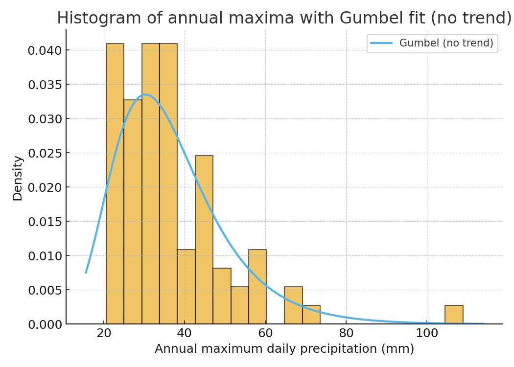
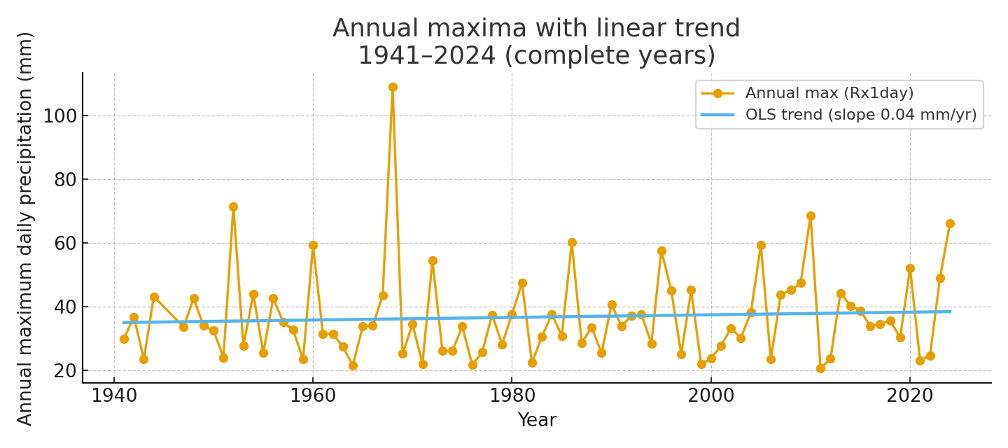
Interpretation (very brief): The histogram checks the no-trend Gumbel fit; the time series shows the OLS trend (mm/year) on annual maxima.
The example shows our results for the German city of Coesfeld. We see a small positive trend in annual maxima of daily rainfalls.
import numpy as np
import pandas as pd
import matplotlib.pyplot as plt
from pathlib import Path

# ===== USER SETTINGS =====
STATION_FILE = "RR_STAID012345.txt"  # change to your station file
START_YEAR = 1941                    # analysis start
MIN_DAYS_PER_YEAR = 330              # completeness (drops partial years like 2025)
OUT_DIR = Path("gumbel_out")
# =========================

GAMMA = 0.5772156649015329  # Euler–Mascheroni
OUT_DIR.mkdir(exist_ok=True, parents=True)

# ---- helpers ----
def detect_header_row(path: Path) -> int:
    lines = path.read_text(encoding="utf-8", errors="ignore").splitlines()
    for i, ln in enumerate(lines[:120]):
        if "SOUID" in ln and "DATE" in ln and "RR" in ln:
            return i
    return 0

def read_ecad_station(path: Path) -> pd.DataFrame:
    hdr = detect_header_row(path)
    df = pd.read_csv(path, skiprows=hdr, header=0)
    df.columns = [c.strip() for c in df.columns]
    keep = [c for c in df.columns if c in ("SOUID","DATE","RR","Q_RR")]
    df = df[keep]
    df["DATE"] = pd.to_datetime(df["DATE"].astype(str), format="%Y%m%d", errors="coerce")
    df["RR"]   = pd.to_numeric(df["RR"], errors="coerce")
    # RR is in 0.1 mm; -9999 means missing
    df["RR_mm"] = df["RR"].where(df["RR"] != -9999, np.nan) / 10.0
    # keep good-quality only (if flag present)
    if "Q_RR" in df.columns:
        df["Q_RR"] = pd.to_numeric(df["Q_RR"], errors="coerce")
        df = df[df["Q_RR"] == 0]
    df["year"] = df["DATE"].dt.year
    return df.dropna(subset=["DATE"])

def latest_complete_year(df: pd.DataFrame, min_days=MIN_DAYS_PER_YEAR):
    counts = df.groupby("year")["RR_mm"].apply(lambda s: s.notna().sum())
    complete = counts[counts >= min_days]
    return None if complete.empty else int(complete.index.max())

def gumbel_mom(sample):
    sample = np.asarray(sample, float)
    m  = float(sample.mean())
    s2 = float(sample.var(ddof=1))
    beta = np.sqrt(6.0 * s2) / np.pi
    mu   = m - GAMMA * beta
    return mu, beta

def gumbel_pdf(z, mu, beta):
    y = (z - mu) / beta
    return (1.0/beta) * np.exp(-(y + np.exp(-y)))

# ---- 1) Read & keep only complete years ----
df = read_ecad_station(Path(STATION_FILE))
if df.empty:
    raise SystemExit("No usable rows after filtering. Check the file.")

last_full = latest_complete_year(df, MIN_DAYS_PER_YEAR)
if last_full is None:
    raise SystemExit("No complete years under the chosen threshold.")

df = df[(df["year"] >= START_YEAR) & (df["year"] <= last_full)].copy()
if df.empty:
    raise SystemExit("No data left in 1941..latest complete year after filtering.")

# ---- 2) Annual maxima ----
annual_max = df.groupby("year")["RR_mm"].max(min_count=1).dropna()
years = annual_max.index.values
x = annual_max.values
t = years - years.min()
n = len(x)

# ---- 3) Fit Gumbel (no trend) + compute OLS trend for series plot ----
mu0, beta0 = gumbel_mom(x)
A = np.vstack([np.ones_like(t), t]).T
coef, *_ = np.linalg.lstsq(A, x, rcond=None)
a_hat, b_hat = float(coef[0]), float(coef[1])

# ---- 4) PLOTS (only two) ----
yr_label = f"{years.min()}–{years.max()} (complete years)"

# 4.1 Histogram + Gumbel fit (no trend)
xs = np.linspace(x.min() - 5, x.max() + 5, 400)
plt.figure(figsize=(7,5))
plt.hist(x, bins=20, density=True, alpha=0.6, edgecolor="black", label="Annual maxima")
plt.plot(xs, gumbel_pdf(xs, mu0, beta0), linewidth=2, label="Gumbel fit (no trend)")
plt.xlabel("Annual maximum daily precipitation (mm)")
plt.ylabel("Density")
plt.title(f"Histogram with Gumbel fit\n{yr_label}")
plt.legend()
plt.tight_layout()
plt.savefig(OUT_DIR / "hist_gumbel_notrend.png", dpi=160)
plt.close()

# 4.2 Time series with OLS trend
plt.figure(figsize=(9,4))
plt.plot(years, x, marker="o", linestyle="-", label="Annual max (Rx1day)")
plt.plot(years, a_hat + b_hat * t, linewidth=2, label=f"OLS trend (slope {b_hat:.2f} mm/yr)")
plt.xlabel("Year")
plt.ylabel("Annual maximum daily precipitation (mm)")
plt.title(f"Annual maxima with linear trend\n{yr_label}")
plt.legend()
plt.tight_layout()
plt.savefig(OUT_DIR / "series_trend.png", dpi=160)
plt.close()

print("Saved:", OUT_DIR / "hist_gumbel_notrend.png", "and", OUT_DIR / "series_trend.png")
print(f"Gumbel (no trend): mu={mu0:.2f} mm, beta={beta0:.2f} mm; OLS slope={b_hat:.3f} mm/yr")
