A Tree-Free Path to Efficiently Compute the Hypervolume Indicator in Three Dimensions

In many algorithmic settings, the use of balanced trees, heaps, or other dynamic data structures is the standard way to achieve good asymptotic complexity. However, these structures can introduce memory fragmentation, unpredictable allocation patterns, garbage collection overhead, and branch-heavy execution — all undesirable in systems where performance must be deterministic and low-level behavior is important. 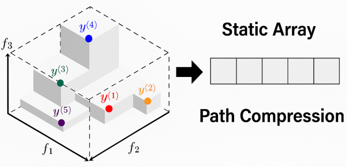For applications such as embedded systems, GPU kernels, or tight inner loops of optimization routines, it is often preferable to rely purely on static arrays with direct indexing. This article shows how the well-known 3-D hypervolume indicator — typically computed with dynamic search trees — can be implemented efficiently in time using only arrays and simple pointer arithmetic.

Efficient exact computation of the 3-D hypervolume indicator (HV) in multiobjective optimization is a well-studied topic. A key milestone is the dimension-sweep approach of Fonseca, Paquete, and López-Ibáñez (2006) for 3-D HV, where a balanced tree maintains the 2-D projection during the sweep. In embedded or performance-sensitive settings (deterministic memory, fewer allocations/GC, predictable constants) we may prefer to avoid dynamic data structures. This post presents a clean array-only algorithm that uses skip pointers with path compression to maintain the 2-D skyline during a single z-sweep. It matches tree-based asymptotics while relying only on arrays, integer indices, and binary search.

Problem Setting (Maximization)

Given a finite set and a reference , the 3-D hypervolume is the union volume of axis-aligned boxes from the origin to each point:

We compute this exactly via a z-sweep (descending ). Between consecutive z-levels, the dominated 2-D area in $(f_1,f_2)$ is constant; multiplying that area by the slab thickness gives the volume contribution.

Algorithm Overview

Z-sweep

Sort distinct -levels in descending order . For each slab , the dominated 2-D area (in ) is constant, and the slab adds to the volume.

2-D projection maintenance (arrays only)

We maintain the 2-D skyline in under maximization (w.r.t. the origin). Implementation-wise, we internally flip signs and work in minimization (see code), but the data structure is the same:

• Fix a static order by (ties by ) to index points .
• Allocate arrays prev_idx[] and next_idx[] (neighbors in that static order) and a boolean active[] to mark skyline membership.
• Insert each point once (when its z-level becomes active), discarding a contiguous run of dominated neighbors on the right and updating the area locally.

Path-compressed skip pointers

Each index in the static -order stores prev_idx[] and next_idx[]. When a node becomes inactive (dominated), we do not physically remove it; lookups must skip it to reach the nearest active neighbor. We apply a simple path compression rule: whenever a lookup traverses an inactive chain, intermediate links are rewired directly to the first active node found. For example:

def find_next_active(pos):
    j = next_idx[pos]
    while j != -1 and not active[j]:
        next_idx[pos] = next_idx[j]   # path compression
        j = next_idx[pos]
    return j

After one such traversal, later lookups from the same position jump directly to the correct active neighbor, bypassing inactives. In practice, each neighbor lookup is effectively constant time on average, because every skipped node is permanently bypassed once it becomes inactive. The structure behaves like a direct-access array—no balanced trees needed.

Area formula (minimization view)

In the minimization variant (used in code via sign flip), if the skyline nodes in ascending are with strictly decreasing , the dominated 2-D area relative to is

All updates when inserting/removing a local run are expressed with differences of these terms, touching only neighbors.

Pseudocode (Core Skeleton)

# Input: points (x,y,z), reference r=(0,0,0) for maximization
# Step 0: sign flip to minimization: (x,y,z) -> (-x,-y,-z), r -> -r
# Step 1: bucket points by z (ascending), tie-break by (x,y)
#         build static Y-order (ascending y; tie x), arrays prev_idx[], next_idx[], active[]
# Step 2: maintain scalar area_2d = 0

# Helpers: find_prev_active / find_next_active using path compression
# Helper: add_node(pos):
#   L = prev active; R = next active
#   if L exists and x[L]  return
#   remove a right run while x[right] >= x_new; adjust area_2d locally
#   add the new node; connect to first kept right; mark active; mark removed as inactive

# Step 3: z-sweep:
#   insert first z-level points with add_node
#   for each slab [z_k, z_{k+1}]: HV += area_2d * (z_{k+1}-z_k); then insert z_{k+1} points

Complexity

Sorting by and the static -order costs . Each point is inserted once; every dominated node is removed at most once overall; skip-pointer path compression makes neighbor search effectively constant on average. Hence total time and memory .

Worked Example (Updated Two Fronts) + Visualization

We replace the old instance with a more varied two-front set (maximization, reference $(0,0,0)$):

We indicate the dominated region (of which the Lebesgue measure is the 3-D Hypervolume indicator) in Figure 2. The exact hypervolume for this instance is:

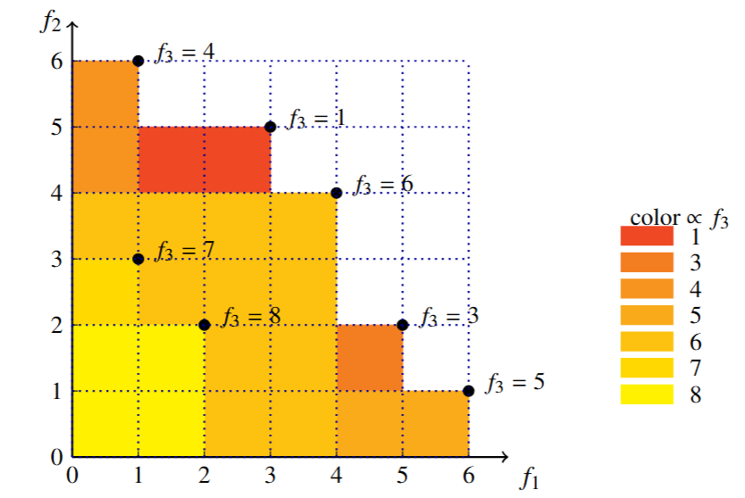
Figure 1: Opaque rectangles from $(0,0)$ to $(f_1,f_2)$, painted in ascending . Black circles mark $(f_1,f_2)$; colors encode .

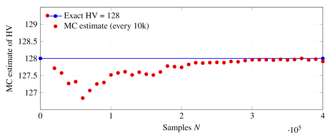
Figure 2. Monte Carlo convergence (every 10k samples up to 400k). Horizontal line marks the exact value .

References

Fonseca, C. M., Paquete, L., & López-Ibánez, M. (2006, July). An improved dimension-sweep algorithm for the hypervolume indicator. In 2006 IEEE international conference on evolutionary computation (pp. 1157-1163). IEEE.

Appendix: Python implementation

The function below computes exact HV in using only arrays and skip pointers (no trees). The example points are the two-front instance above. A Monte Carlo script (uniform within the bounding box ) is included for sanity checking.

Implementation note: All data structures are fixed-size arrays; the skip-pointer traversal uses path compression so subsequent neighbor lookups become effectively constant-time on average. No balanced trees or heaps are used.

CITE ME AS:

Emmerich, M. T. M. (2025, October 5). A tree-free path to efficiently compute the hypervolume indicator in three dimensions [Blog post, Multiobjective Optimization and Decision Analyis News]. http://www.emmerix.net.

from collections import defaultdict

def hypervolume_3d_min_arrays(points, ref):
    """
    3-D hypervolume (minimization) via z-sweep and a 2-D skyline in (x,y),
    implemented with static arrays and skip pointers (no trees).
    """
    rx, ry, rz = map(float, ref)

    # Filter to ref-box and stabilize order
    P = [(float(x), float(y), float(z)) for (x, y, z) in points
         if x <= rx and y <= ry and z <= rz]
    if not P:
        return 0.0

    n = len(P)
    xs = [p[0] for p in P]
    ys = [p[1] for p in P]

    # Bucket by z (ascending); tie-break within a level by (x,y)
    by_z = defaultdict(list)
    for i, (x, y, z) in enumerate(P):
        by_z[z].append(i)
    z_levels = sorted(by_z.keys())
    for z in z_levels:
        by_z[z].sort(key=lambda i: (xs[i], ys[i]))

    # Static Y-order (ascending y; tie-break by x)
    ordY = sorted(range(n), key=lambda i: (ys[i], xs[i]))
    posY = [0]*n
    for p, i in enumerate(ordY):
        posY[i] = p

    # Skip-pointer arrays over Y-order
    prev_idx = [i-1 for i in range(n)]
    next_idx = [i+1 for i in range(n)]
    prev_idx[0] = -1
    next_idx[-1] = -1
    active = [False]*n

    def x_at(pos):  # multi-use
        return xs[ordY[pos]]

    def y_at(pos):  # multi-use
        return ys[ordY[pos]]

    def find_prev_active(pos):  # multi-use
        j = prev_idx[pos]
        if j == -1:
            return -1
        while j != -1 and not active[j]:
            prev_idx[pos] = prev_idx[j]
            j = prev_idx[pos]
        return j

    def find_next_active(pos):  # multi-use
        j = next_idx[pos]
        if j == -1:
            return -1
        while j != -1 and not active[j]:
            next_idx[pos] = next_idx[j]
            j = next_idx[pos]
        return j

    area_2d = 0.0  # sum over active pos: (x_prev(pos) - x[pos]) * (ry - y[pos])

    def add_node(pos):  # multi-use
        nonlocal area_2d
        x_new = x_at(pos)
        y_new = y_at(pos)

        L = find_prev_active(pos)
        R = find_next_active(pos)

        # If dominated by left active (x_left <= x_new), ignore
        if L != -1 and x_at(L) <= x_new:
            return

        # Remove consecutive right run with x >= x_new
        removed = []
        R_it = R
        while R_it != -1 and x_at(R_it) >= x_new:
            removed.append(R_it)
            R_it = find_next_active(R_it)
        R_keep = R_it  # first right node with x < x_new (or -1)

        # Decrement area: old edge into R_keep
        if R_keep != -1:
            x_prev_old = (x_at(removed[-1]) if removed else (x_at(L) if L != -1 else rx))
            area_2d -= (x_prev_old - x_at(R_keep)) * (ry - y_at(R_keep))

        # Decrement area: contributions of removed block
        if removed:
            x_prev = x_at(L) if L != -1 else rx
            for rpos in removed:
                area_2d -= (x_prev - x_at(rpos)) * (ry - y_at(rpos))
                x_prev = x_at(rpos)

        # Add area: new node + new edge to R_keep
        xL = x_at(L) if L != -1 else rx
        area_2d += (xL - x_new) * (ry - y_new)
        if R_keep != -1:
            area_2d += (x_new - x_at(R_keep)) * (ry - y_at(R_keep))

        # Activate new, deactivate removed
        active[pos] = True
        for rpos in removed:
            active[rpos] = False

    # ---- z-sweep ----
    hv = 0.0

    # Insert first z level
    first_z = z_levels[0]
    for i in by_z[first_z]:
        add_node(posY[i])

    # Process slabs
    for k in range(len(z_levels)):
        z_cur = z_levels[k]
        z_next = rz if k+1 == len(z_levels) else z_levels[k+1]
        hv += area_2d * (z_next - z_cur)
        if k+1 &lt; len(z_levels):
            for i in by_z[z_levels[k+1]]:
                add_node(posY[i])

    return hv

def hypervolume_3d_max(points, ref=(0.0,0.0,0.0)):
    # Reduce maximization to minimization by negation
    neg_points = [(-x, -y, -z) for (x,y,z) in points]
    neg_ref = (-ref[0], -ref[1], -ref[2])
    return hypervolume_3d_min_arrays(neg_points, neg_ref)

if __name__ == "__main__":
    # Updated example (two fronts)
    P = [(1,6,4), (3,5,1), (4,4,6), (5,2,3), (6,1,5), (1,3,7), (2,2,8)]
    print("Exact HV:", hypervolume_3d_max(P, (0,0,0)))  # 128.0

def hv_monte_carlo(points, N=400_000, step=10_000):
    maxx = max(x for x,_,_ in points)
    maxy = max(y for _,y,_ in points)
    maxz = max(z for *_,z in points)
    Vbox = maxx * maxy * maxz

    def covered(x,y,z, pts):
        for (px,py,pz) in pts:
            if x <= px and y <= py and z <= pz:
                return True
        return False

    random.seed(42)
    cnt = 0
    series = []  # (N, estimate)
    for i in range(1, N+1):
        x = random.random() * maxx
        y = random.random() * maxy
        z = random.random() * maxz
        if covered(x,y,z, points):
            cnt += 1
        if i % step == 0:
            est = Vbox * (cnt / i)
            series.append((i, est))
    return series  # plot these pairs

if __name__ == "__main__":
    P = [(1,6,4), (3,5,1), (4,4,6), (5,2,3), (6,1,5), (1,3,7), (2,2,8)]
    print(hv_monte_carlo(P))