The Tent Map – A Simple Path to Chaos

Michael Emmerich, August 20th 2025

Chaotic time series can emerge from very simple deterministic rules. The tent map is a classical example. It shows how fixed points can be unstable, how orbits diverge, and how randomness-like behavior arises from a piecewise linear rule.

The Tent Map

The tent map is defined on the interval ${[0,1]}$ by

$\displaystyle T(x) = \begin{cases} \mu x, & 0 \leq x < 1/2, \\ \mu (1-x), & 1/2 \leq x \leq 1 , \end{cases}$

with parameter ${0 \leq \mu \leq 2}$ . For ${\mu=2}$ , the system is chaotic.

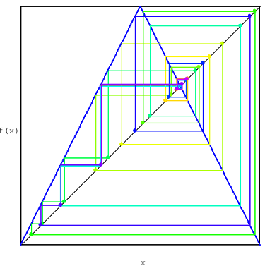
The reader is encouraged to examine Figure 1, which provides a visualization of the cobweb plot together with the corresponding time series. Standard references on cobweb diagrams and the theory of interval maps have been included at the end of this essay. For those interested in a deeper exploration, we invite the reader to experiment with the interactive Python source code provided in the appendix.

Fixed Points and Instability

A fixed point ${x^*}$ satisfies ${T(x^*)=x^*}$ . The derivative is

$\displaystyle T'(x) = \begin{cases} \mu, & 0 \leq x < 1/2, \\ -\mu, & 1/2 \leq x \leq 1 . \end{cases}$

If ${|T'(x^*)|<1}$ the fixed point attracts nearby orbits. If ${|T'(x^*)|>1}$ it repels them. For ${\mu=2}$ , both fixed points are repelling. Orbits starting close to a fixed point are pushed away, and nearby trajectories separate exponentially fast.

Cobweb Visualization

A cobweb diagram shows iterations graphically. Starting from some ${x_0}$ , each step alternates between the curve ${y=T(x)}$ and the diagonal ${y=x}$ . For ${\mu=2}$ the orbit never settles but explores the interval irregularly, sensitive to the initial condition.

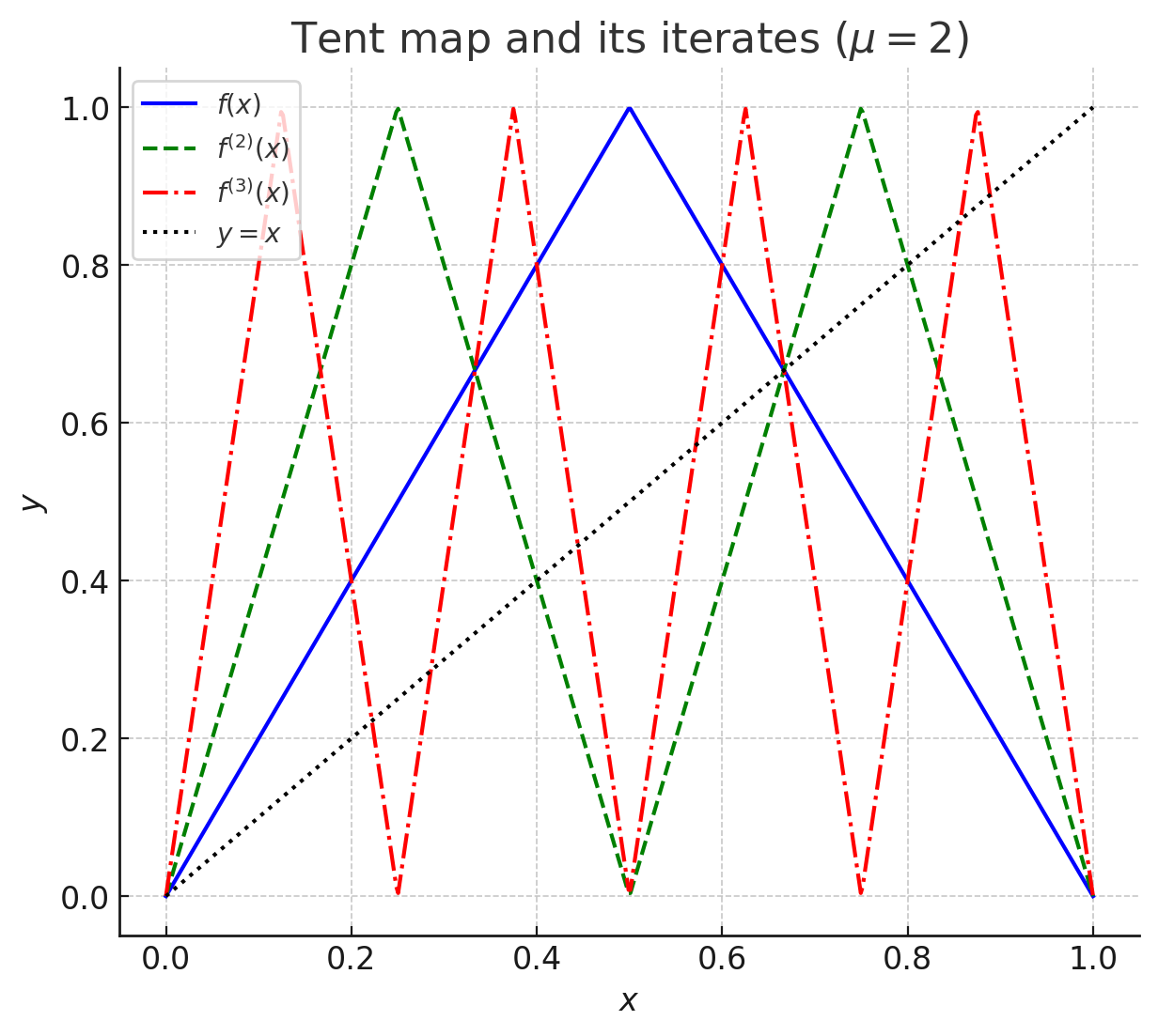
Periodic Points and Higher Iterates

An orbit of period ${k}$ is a point where ${T^k(x)=x}$ , where ${T^2(x) = T(T(x)), T^3(x)=T(T(T(x)))}$ , and so on. The ${k}$ -th iterate of ${T}$ , denoted ${T^{(k)}}$ , has many such points, as can be seen in Figure 3 (intersections with diagonal). As ${k}$ increases, the number of periodic points grows quickly, showing how densely chaos fills the interval.

Invariant Density and Lyapunov Exponent

Iterating the tent map produces a long-term distribution called the invariant density. For ${\mu=2}$ , it is uniform on ${[0,1]}$ :

$\displaystyle \rho(x) = 1, \quad 0 \leq x \leq 1.$

This means the orbit spends equal amounts of time in each part of the interval. The Lyapunov exponent measures how fast nearby orbits diverge. For ${\mu=2}$ it equals ${\ln(2)}$ , which is positive. A positive Lyapunov exponent confirms sensitivity to initial conditions, a typical characteristic of deteministic chaos dynamics.

The Binary Shift Map Connection

The tent map with ${\mu=2}$ is topologically conjugate to the binary shift map

$\displaystyle S(x)=2x \pmod{1}, \quad x \in [0,1].$

If ${x=0.a_1a_2a_3\ldots}$ in binary, then one step of ${S}$ simply shifts the digits:

$\displaystyle S(x)=0.a_2a_3a_4\ldots.$

Each iteration discards the first digit. This shows that the tent map and the binary shift share the same chaotic structure. Iterating them resembles tossing a fair coin.

For rational numbers ${x=p/q}$ with denominator ${q=2^a m}$ (with ${m}$ odd), the orbit under ${S}$ is eventually periodic. After ${a}$ steps the factor ${2^a}$ is removed, and the period is the multiplicative order of ${2}$ modulo ${m}$ . For ${q}$ prime, the period always divides ${q-1}$ , and is maximal when ${2}$ is a primitive root modulo ${q}$ .

Another way to describe periodicity is that points of exact period ${n}$ are rationals of the form

$\displaystyle x=\frac{k}{2^n-1}, \quad k=0,1,\ldots,2^n-2.$

These correspond to primitive binary blocks of length ${n}$ , linking dynamics with combinatorics of binary sequences.

Chaos and Number Theory

The connection between the tent map and the binary shift hints at deeper parallels with number theory. The tent map has a dynamical zeta function encoding periodic orbits, while number theory studies the Riemann zeta function, which encodes the primes. In both cases, apparent randomness emerges from deterministic rules. Chaos in dynamics and irregularity in primes may thus be seen as two sides of pseudorandomness. We would like to futher explore this connection and provide more details on the binary shift map in a future blog post.

Conclusion

The tent map, though defined by a simple formula, displays chaos: repelling fixed points, exponential divergence, dense periodic orbits, and uniform distribution. Its link with the binary shift map shows how deterministic systems can mimic random behavior, much like the distribution of prime numbers.

P. Collet and J.-P. Eckmann. Iterated Maps on the Interval as Dynamical Systems. Birkhäuser, Boston, 1980.
R. L. Devaney. An Introduction to Chaotic Dynamical Systems. 2nd edition, Addison-Wesley, Redwood City, CA, 1989.

Figure 1:

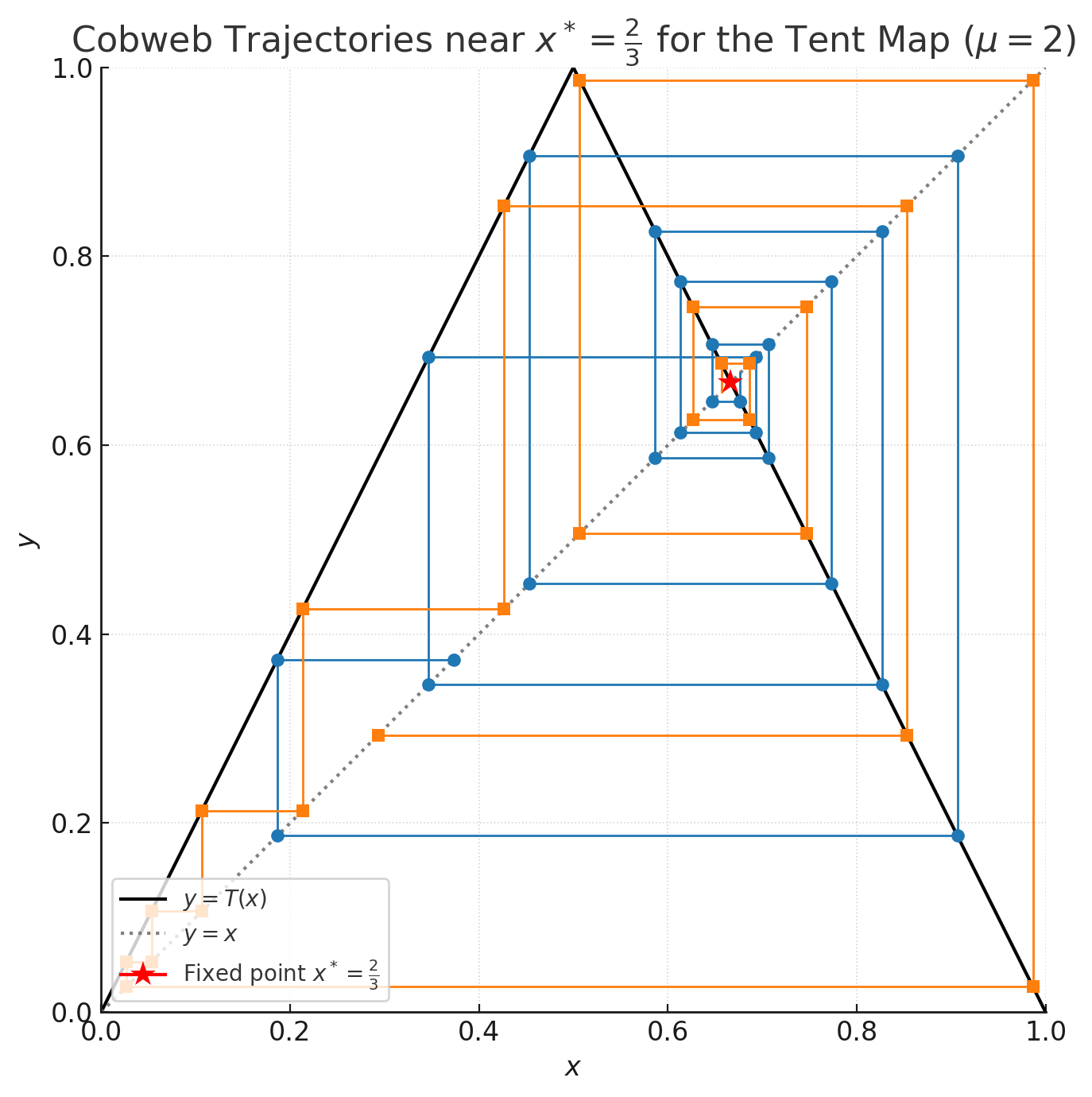
Figure 2:

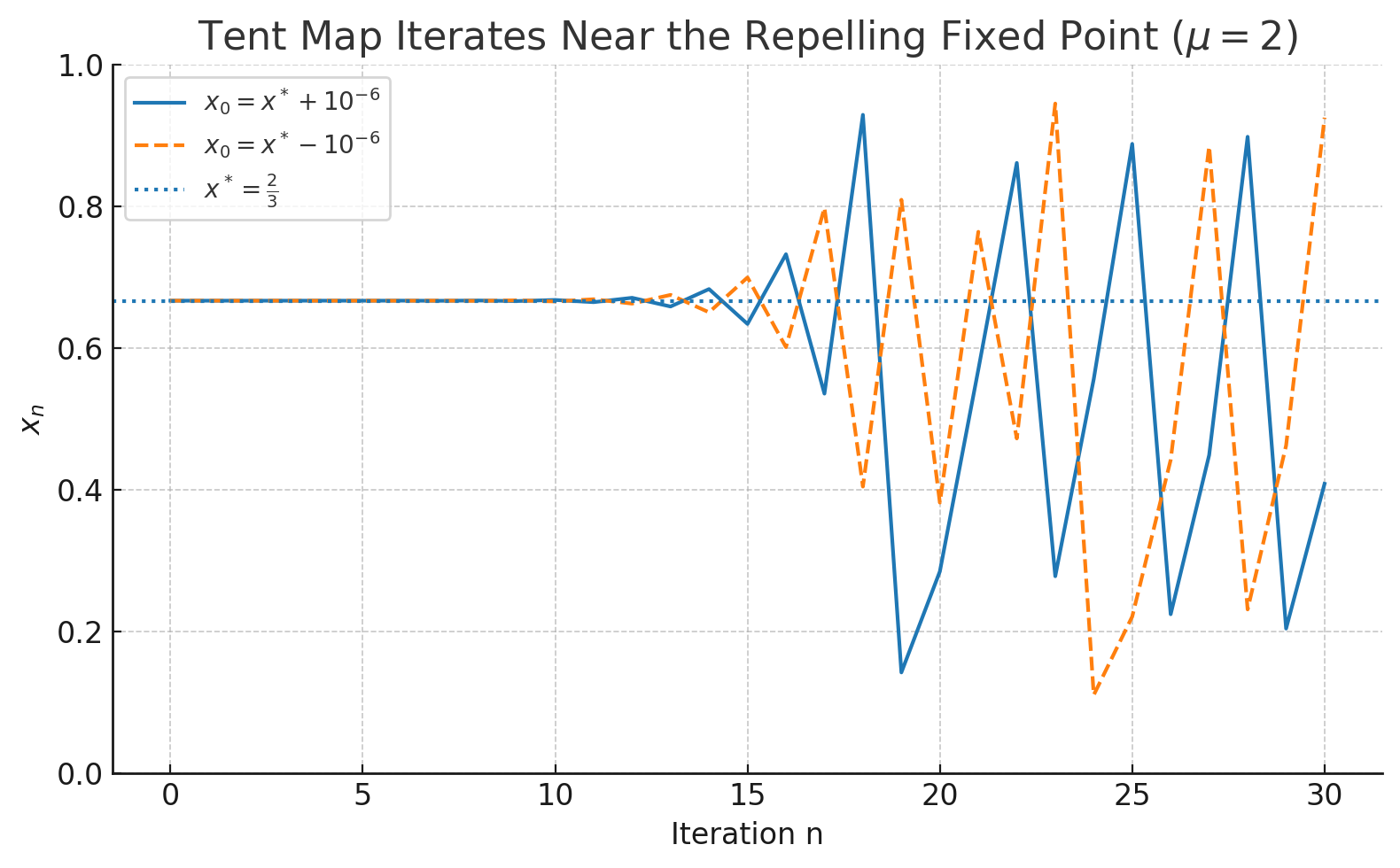
Figure 3

Interactive Python Source code on Trinket.io:
https://trinket.io/library/trinkets/077d82abad0b

The Tent Map – A Simple Path to Chaos

Share this:

Leave a comment Cancel reply