Michael Emmerich, January 16th, 2025
(inspired by a discussion of an application problem with Jonas Schwaab, ETH Zurich)
In single-objective optimization, it is easy to visualize a function that depends on only two continuous or integer input variables by means of a heatmap plot, where the lightness indicates the achievement in the objective function, say F(x1, x2), for input values, say x1 and x2. When we have two or multiple conflicting objective functions, say F1(x1,x2) and F2(x1,x2), this becomes a challenge: Plots have been suggested that measure the volume of the dominated subspace (Fonseca, 1995) and others that look at the angle between the gradients of the objective functions (Schäpermeier et al., 2020). Here we present a new idea, which is simple to implement and has a straightforward definition of proximity to the Pareto front.
This post presents a heatmap visualization for multiobjective optimization, illustrating Pareto dominance and epsilon dominance between two conflicting objective functions:
where, considering maximization and objectives normalized from zero (lowest achievement) to one (top achievement):
- F1(i, j) represents the achievement in one objective.
- F2(i, j) represents the achievement in another conflicting objective.
- Epsilon dominance measures how much improvement is needed (epsilon added to both objective function value) such that the vector becomes non-dominated.
Visualization Goals
- Color representation:
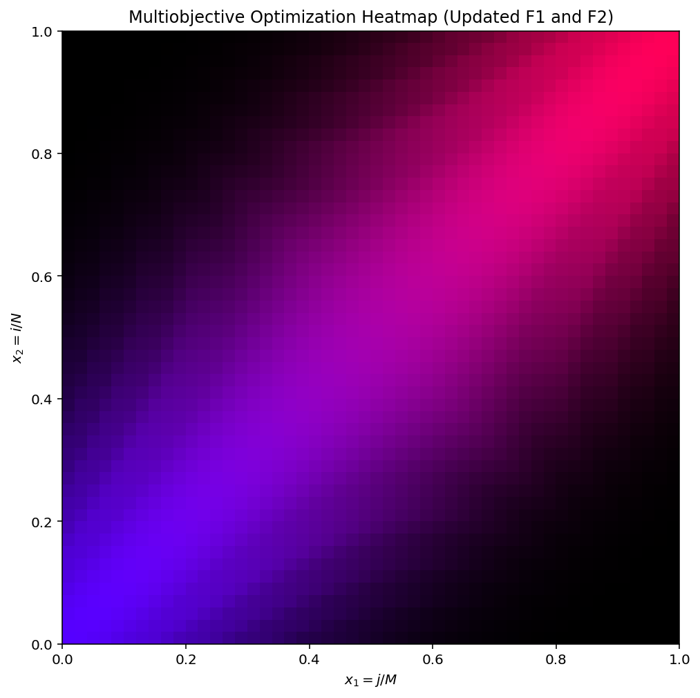
- Blue intensity is proportional to achievement in F1.
- Red intensity is proportional to achievement in F2.
- Lightness is inversely proportional to epsilon dominance (more dominance means darker color).
An example of a simple problem with a linear Pareto efficient set ranging from 0 to 1 is given in the first plot example.


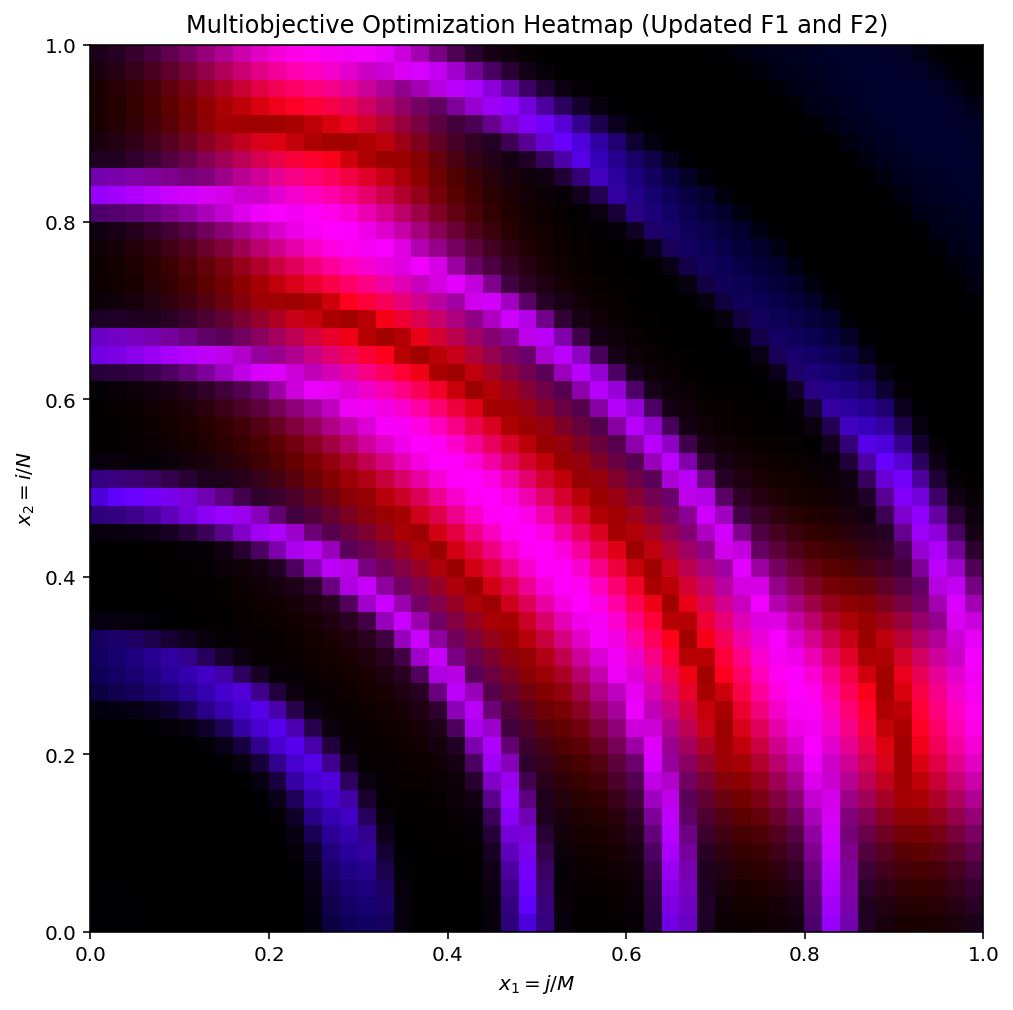
The second example shows the result for a multimodal function with many local optima.


Implementation in Python
Below is the full Python script used to generate the heatmap:
import numpy as np
import matplotlib.pyplot as plt

# Define parameters
M, N = 50, 50  # Matrix dimensions

# Define new objective functions
F1 = 1 / (1 + (np.arange(M)[:, None] / N) ** 2 + (np.arange(N)[None, :] / M) ** 2)
F2 = 1 / (1 + (np.arange(M)[:, None] / N - 1) ** 2 + (np.arange(N)[None, :] / M - 1) ** 2)

# Multimodal complex multiobjective problem
# F1 = (np.sin(29*1 / (1 + (np.arange(M)[:, None] / N) ** 2 + (np.arange(N)[None, :] / M) ** 2)))**2
# F2 = (np.cos(5*1 / (1 + (np.arange(M)[:, None] / N - 1) ** 2 + (np.arange(N)[None, :] / M - 1) ** 2)))**2


# Compute Pareto front
pareto_mask = np.ones((M, N), dtype=bool)

for x2 in range(M):
    for x1 in range(N):
        for k in range(M):
            for l in range(N):
                if (F1[k, l] >= F1[x2, x1] and F2[k, l] >= F2[x2, x1]) and (F1[k, l] > F1[x2, x1] or F2[k, l] > F2[x2, x1]):
                    pareto_mask[x2, x1] = False
                    break
            if not pareto_mask[x2, x1]:
                break

# Compute Epsilon dominance values for dominated points
Eps = np.zeros((M, N))

for x2 in range(M):
    for x1 in range(N):
        if not pareto_mask[x2, x1]:  # If dominated
            min_eps = float('inf')
            for k in range(M):
                for l in range(N):
                    if pareto_mask[k, l]:  # Check against Pareto-optimal points
                        eps1 = max(0, F1[k, l] - F1[x2, x1])
                        eps2 = max(0, F2[k, l] - F2[x2, x1])
                        min_eps = min(min_eps, max(eps1, eps2))
            Eps[x2, x1] = min_eps if min_eps != float('inf') else 0

# Normalize Eps for color lightness scaling
Eps_normalized = Eps / np.max(Eps) if np.max(Eps) > 0 else Eps

# Generate colormap (red for F2, blue for F1, intensity by Eps)
heatmap = np.zeros((M, N, 3))
heatmap[:, :, 0] = F2  # Red channel (F2 achievement)
heatmap[:, :, 2] = F1  # Blue channel (F1 achievement)

# Scale by lightness (Eps intensity)
lightness = (1 - Eps_normalized)**4  # Higher epsilon should be lighter
heatmap = heatmap * lightness[:, :, np.newaxis]

# Plot heatmap
plt.figure(figsize=(8, 8))
x1_vals = np.linspace(0, 1, N)  # x-axis from j/M
x2_vals = np.linspace(0, 1, M)  # y-axis from i/N
plt.imshow(heatmap, origin='lower', extent=[0, 1, 0, 1], aspect='auto')
plt.xlabel('$x_1 = j/M$')
plt.ylabel('$x_2 = i/N$')
plt.title('Multiobjective Optimization Heatmap (Updated F1 and F2)')
plt.show()
Interpretation of Results
- Blue areas indicate strong achievement in F1.
- Red areas indicate strong achievement in F2.
- Light-colored areas represent non-dominated or weakly dominated solutions.
- Dark-colored areas indicate strong dominance (high epsilon values), requiring larger improvement to become Pareto-optimal.
Discussion and Further Reading
This visualization showcases trade-offs in multiobjective optimization through a heatmap that highlights Pareto dominance and epsilon dominance as a proximity indicator to Pareto efficiency, aiding in the analysis of multimodal multiobjective landscapes.
Applications include decision support in optimization, visualization of trade-offs in multi-criteria decision-making, and analysis of competitive objectives in spatial location planning.
In Schäpermeier 2020 alternative ways to plot proximity to Pareto efficiency are discussed. The idea of this plot to use epsilon-dominance as a proximity indicator to Pareto efficiency is in a simpler version realized for a visualization of the multiobjective Himmelblau function level set in Pereverdieva et al. 2024.
References
Fonseca, C.M.M.: Multiobjective genetic algorithms with application to control engineering problems. Ph.D. Thesis, Department of Automatic Control and Systems Engineering, University of Sheffield, September 1995
Schäpermeier, L., Grimme, C., & Kerschke, P. (2020, September). One PLOT to show them all: visualization of efficient sets in multi-objective landscapes. In International Conference on Parallel Problem Solving from Nature (pp. 154-167). Cham: Springer International Publishing.
Pereverdieva, K., Deutz, A., Ezendam, T., Bäck, T., Hofmeyer, H., & Emmerich, M. (2024). Comparative Analysis of Indicators for Multiobjective Diversity Optimization. arXiv e-prints, arXiv-2410. (To appear in EMO 2025 Proceedings)
