Of Autumn Leaves and Coupon Collectors

Essay by Michael Emmerich, October 11th, 2024

Imagine a peaceful autumn day where leaves gently fall, covering a patch of land. The land can be represented as a grid or matrix with distinct places, each starting uncovered. As the leaves fall, they randomly land on one of these places, gradually covering the ground. But how long will it take for the entire patch of land to be fully covered with leaves? Please let your self get inspired by our interactive source code demo of this random process:

Link to Maple Leaves Interactive Source Code Demo (trinket.io)

This situation mirrors a common computational problem where we start with a bit string of length , all bits initialized to 0. Each step represents a random flip of a bit from 0 to 1, analogous to a leaf covering an uncovered spot. Our goal is to figure out the expected number of flips (or fallen leaves) required to flip every bit to 1 (or cover every place on the patch of land).

The process of covering all places behaves similarly to the well-known coupon collector’s problem. Initially, every leaf that falls is guaranteed to cover a new spot. However, as more spots are covered, the likelihood of a leaf landing on an already-covered place increases. This creates a pattern where fewer uncovered spots remain over time, making it progressively harder to cover the remaining spots.

Lemma 1

Let be the number of spots (or bits) on the grid. At each step, a leaf falls randomly onto one of the uncovered spots (flipping a bit from 0 to 1). The expected number of steps needed to fully cover the grid (or flip all bits to 1) is:

where is the -th harmonic number.

For large , the harmonic number is approximately:

where is the Euler-Mascheroni constant. (This constant is an interesting object of study in its own sake and there are open mathematical questions related to it, e.g., whether or not it is a rational number.) Therefore, the expected number of steps to cover all spots is approximately:

Thus, for large , the expected number of steps required is roughly , with a small additive constant due to .

Proof: We consider the number of steps required to flip all bits from 0 to 1. Initially, all bits are 0, so the first bit flip is guaranteed to flip a 0 to a 1. On average, this takes 1 step. After one bit is flipped, bits remain at 0, so the probability of flipping another 0 in the next step is . The expected number of steps to flip this second bit is .

In general, after bits have been flipped, bits remain at 0, and the probability of flipping another 0 is . The expected number of steps to flip the -th bit is therefore .

Thus, the total expected number of steps to flip all bits is the sum:

where is the harmonic number. This concludes the proof.

Expected Number of Uncovered Spots Over Time

At step , the probability that a new leaf covers an uncovered spot decreases as more spots are already covered. The expected number of uncovered spots after steps is:

This formula describes an exponential decay, where the number of uncovered spots decreases over time as leaves continue to fall.

Visualization

The following plot illustrates the dynamics of this process, showing how the number of uncovered spots decreases as leaves continue to fall. As seen, the number of uncovered spots decreases rapidly at first but slows down as fewer uncovered spots remain. This is typical behavior predicted by the coupon collector’s problem.

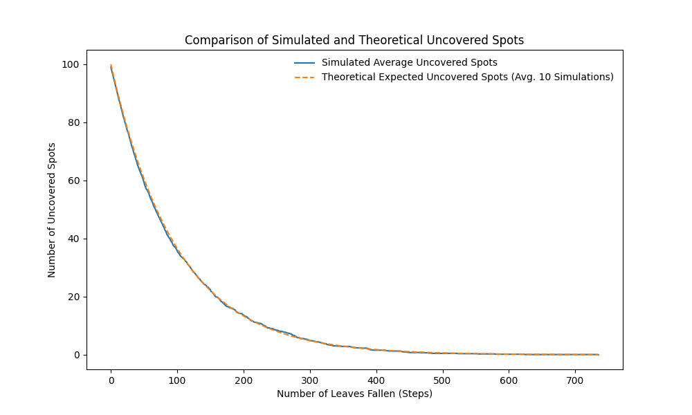
Figure 1Comparison of Simulated and Theoretical Expected Uncovered Spots. The solid line represents the simulated average number of uncovered spots over time, while the dashed line shows the theoretical expectation.

The Coupon Collector problem was made popular by William Feller (see references) under that name but has been studied earlier by mathematicians. It has many applications throughout mathematics of stochastic systems. Notably, it is even related to our perception of the flow of time, as we perceive time to proceed faster when similar events are repeating.

William Feller’s “An Introduction to Probability Theory and Its Applications” (first published in 1950)

Appendix (python code to produce the plot):

import numpy as np
import matplotlib.pyplot as plt
# Simulation parameters
n = 100  # Number of places (size of the patch of land)
trials = 10  # Number of simulations to average the results
# Function to simulate the process
def simulate_leaves_falling(n):
    uncovered_spots = n
    steps = 0
    uncovered_history = []
    covered = np.zeros(n)  # All spots are initially uncovered
    while uncovered_spots > 0:
        # Randomly pick a place and cover it
        place = np.random.randint(0, n)
        if covered[place] == 0:  # If the place is uncovered
            covered[place] = 1  # Cover it
            uncovered_spots -= 1
        uncovered_history.append(uncovered_spots)
        steps += 1

    return uncovered_history
# Average results over multiple trials
max_steps = 0
all_simulations = []
for _ in range(trials):
    result = simulate_leaves_falling(n)
    all_simulations.append(result)
    max_steps = max(max_steps, len(result))

# Align results by padding shorter simulations with the last value
for i in range(len(all_simulations)):
    all_simulations[i] = np.pad(
        all_simulations[i], (0, max_steps - len(all_simulations[i])),
        'edge'
    )
# Compute the average uncovered spots at each step
avg_uncovered = np.mean(all_simulations, axis=0)

# Formula for theoretical uncovered spots:
# E[uncovered spots at t] = n * (1 - 1/n)^t
theoretical_uncovered = [
    n * (1 - 1 / n) ** t for t in range(max_steps)
]
# Plot both the simulation results and the corrected theoretical curve
plt.figure(figsize=(10, 6))
plt.plot(
    avg_uncovered, label="Simulated Average Uncovered Spots"
)
plt.plot(
    theoretical_uncovered,
    label="Theoretical Expected Uncovered Spots (Avg. 10 Simulations)",
    linestyle='--'
)
plt.title(
    "Comparison of Simulated and Theoretical Uncovered Spots"
)
plt.xlabel("Number of Leaves Fallen (Steps)")
plt.ylabel("Number of Uncovered Spots")
plt.grid(False)
plt.legend(loc='upper right', frameon=False,)
# Save the plot as a PNG file
plt.savefig("C:\\Users\\emmer\\Downloads\\dynamic_plot_plus.png")
plt.show()