Grand Cycles of the Primes

On Periodic Patterns in the Prime Clockwork – September 15th, 2024, Michael Emmerich

I have two rotating gears, with 90 and 54 teeth. When do the starting points of these gears align?

— Wilson, R. (2020). Number Theory: A Very Short Introduction. Oxford University Press, Page 7

When do the gears align again? The textbook answer is the least common multiple—though for two gears, their alignment is simply the product of their teeth, if and only if those gears are coprime. This mechanical precision can even define what it means to be prime. In this essay, we visit the clockwork of prime cycles, which generates integers and primes not by traditional means of divisibility or multiplication, but by following a method that generates the configurations of the cog wheels step-by-step, where each move generates a new configuration until all possible configurations were encountered and the wheels are aligned again.

This essay builds on the theories of the ‘prime clockwork’ and ‘prime vectors’ by focusing on recurring modulus combinations. It proves an upper bound for prime density and shows integer factorizations as zeros of a complex function, offering a visualization of the prime clockwork which we will present as interactive python code.

The prime clockwork ( Emmerich24b) is an automaton that generates integers one-by-one in their prime factorization. It uses the metaphor of an array of different clocks, each congruent with a prime number. As a whole, the prime clockwork generates the integers (total seconds that have passed) starting from one, step-by-step as prime vectors, that is, in their unique integer factorization. The prime clockwork uses only integer addition and comparisons, avoiding division and multiplication and each subsequent state of the clockwork depends solely on the preceding state. 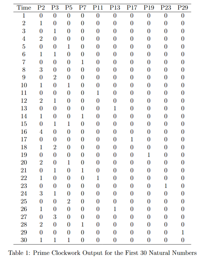We can depict the output of the prime clockwork as a table (See Table 1), each row representing an integer, and each column associated with a prime ${p_i}$ and showing the exponents of the prime factorization of that integer. Alternatively, we may just look at the congruences (moduli) of the integer with the primes (Table 3). These are the analogues of second counters for clocks, that turn around not in 60 seconds, but in ${p_i}$ seconds. Iterating over the rows (associated with the natural numbers or the seconds that have passed) we aim to find and confirm periodic patterns over subsets of columns (each column associated with a prime number exponent in the prime factorization or modulus), detailing their nature and lengths.

In this essay will discuss the following topics:

Subsets of Columns and Long Cycles: Fixing columns tied to prime moduli creates long cycles of repeated configurations over time.
Cycle Length: The length of these cycles is exactly the product of the primes associated with the selected columns.
Combination of modulus values (‘second counters’): Within each long cycle, the seconds counters ${ s_i }$ with ${t \equiv s_i \mod p_i}$ of the prime clocks go through all possible combinations.
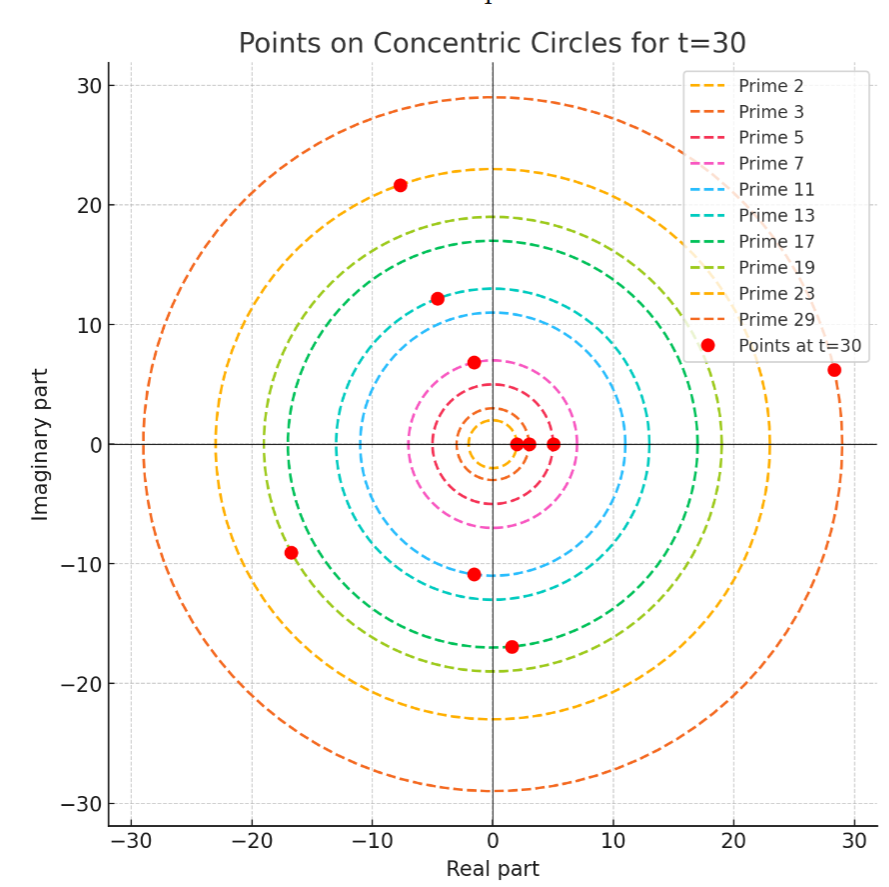
Visualization of Prime Clocks as Complex Functions: Representing the clockwork with time dependent exponential functions with complex exponents (that appear in the plot as concentric circles) represents the prime clockwork as points orbiting the origin at a radius that is proportional to the defining prime number of a clock; all points move with exactly the same speed. Each alignment of points with the positive real axis of a subset of prime clocks marks the end of a long periodic cycle, revealing prime factor of the integer that represents the given time.

The concept of prime vectors and prime clockwork offers a different perspective on integers and prime numbers. While the theoretical results might not all new in the well researched field of number theory, we hope that the new perspective can offer some new ideas. We are certainly inspired by number theory’s rich history but we develop lemmas from basic principles and prefer to build theories up from scratch using elementary methods, driven by curiosity. Please leave a comment to reference related work or identify errors.

1. Prime Vectors

Prime vectors, introduced for instance in Emmerich 2024a represent ${p}$ -adic orders as tuples in a positional notation and play an essential role in the definition of the prime clockwork. For ${ z \in \mathbb{N} }$ , represent ${ z }$ as ${ z = \prod_{i=1}^\infty p_i^{k_i} }$ , where ${ p_i }$ are primes and ${ k_i \in \mathbb{N}_0 }$ . We define a prime vector as an infinite list ${ p = (k_1, k_2, \dots) }$ . The mapping between integers and prime vectors is ${ P(z) }$ , with the inverse ${ P^{-1}(z) }$ . The space of prime vectors is ${ \mathbb{P} }$ . Define the ${\odot}$ operator on ${ \mathbb{P} }$ as ${ a \odot b = (a_1 + b_1, a_2 + b_2, \dots) }$ , and observe that ${P^{-1}(a \odot b) = P^{-1}(a) \cdot P^{-1}(b)}.$

2. Prime Clockwork

The prime clockwork was introduced earlier in this blog
Emmerich 2024b.

Definition 1 A prime clock for prime ${ p_i }$ , denoted ${ \circledast(p_i, t) }$ , is a recursive automaton starting at ${ t = 1 }$ and generating an output ${ o_i(t) \in \mathbb{N}_0 }$ each iteration. It has a seconds counter ${ s_i(t) }$ that is increased by one in each iteration and reset to ${ 0 }$ before it reaches ${ p_i }$ , i.e., it holds ${ s_i(t) = t \bmod p_i }$ . It has a minutes counter ${ m_i(t) }$ that starts with ${ m_i(1) = 0 }$ and increases by one after each reset of the seconds counter. The prime clock outputs ${ o_i(t) = o_i(m_i(t)) + 1 }$ whenever ${ s_i(t) = 0 }$ , and ${ o_i(t) = 0 }$ otherwise.

Definition 2 The dynamic prime clockwork starts with only one active prime clock in the array, the prime clock for ${ p_1 = 2 }$ . As the counting process progresses, new prime clocks ${ \circledast(p_{i+1},.) }$ are activated and added with ${ p_{i+1} = t_0 }$ when all active prime clocks output ${ 0 }$ simultaneously for the first time, which implies ${ t_0 }$ is a prime number.

We use the term dynamic prime clockwork, if we want to emphasize that prime numbers are generated on the fly. Otherwise, we just use the term prime clockwork.

3. Grand cycles

Although the process of generating primes is known for its irregularity, there are processes the prime clockwork performs that perform long cycles of periodically repeated patterns. Let us have a closer look at these.

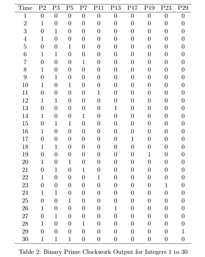
Definition 3 {Binary Prime Clockwork} Let us define a simplification of the output of the prime clockwork with outputs ${o_i(t)}$ (prime factor exponents) as follows.
$\displaystyle b_i(t) = \begin{cases} 0 &\text{if } o_i(t) = 0 \\ 1 &\text{otherwise} \end{cases}$
Similarly to prime vectors ${P(t)}$ , we refer to the result of these sequences as binary prime vectors, which we represent by ${B(t)}$ .

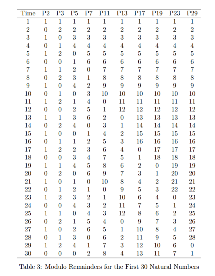
Please see an example of the (binary) prime clockwork output for the integers from 1 to 30 in the Table 1 and Table 2 (for the binary clockwork). The modulo remainders for the primes defining the columns are listed in Table 3, and we will discuss them later on.

Remark 1 The sequence of ${b_i(t)}$ could be simulated correctly without computing ${o_i(t)}$ by a simplified dynamic clockwork.

Remark 2 This abstraction of the prime clockwork output serves two purposes:

The appearance of new primes relies only on the presence of ${0}$ s in the output, and consequently, the exponents in the prime factorizations may be of little importance for questions regarding the distribution of the primes.
The sequences ${b_i(t)}$ repeat subsequences, unlike ${o_i(t)}$ .

Now, let us examine the characteristics and duration of the recurring sequences.

Lemma 1 Let ${ \{i_1, \dots, i_k\} \subset \mathbb{N} }$ be a subset of natural numbers. Consider the rows of the prime clockwork table indexed by time ${ t }$ , denoted ${ B(t) }$ , and let ${ B(t)_{\{i_1, \dots, i_k\}} }$ represent the projection of ${ B(t) }$ onto the columns corresponding to the indices ${ \{i_1, \dots, i_k\} }$ .
The sequence ${ B(t)_{\{i_1, \dots, i_k\}} }$ is periodic with period ${ T = \prod_{j=1}^{k} p_{i_j} }$ , where ${ p_{i_j} }$ are the primes associated with the indices ${ i_j }$ . Specifically, for all ${ t \geq 1 }$ ,
$\displaystyle B(t)_{\{i_1, \dots, i_k\}} = B(t + T)_{\{i_1, \dots, i_k\}}.$
In other words, the sequence ${ B(t)_{\{i_1, \dots, i_k\}} }$ repeats itself every ${ T }$ iterations, starting from ${ t = 1 }$ .

Proof: The seconds counters ${ s_{i_j}(t) }$ for each prime clock ${ p_{i_j} }$ reset to zero simultaneously exactly when ${ t }$ is a multiple of ${ \prod_{j=1}^{k} p_{i_j} }$ . This marks the start of a new cycle where the sequence ${ B(t)_{\{i_1, \dots, i_k\}} }$ repeats. Since the behavior of each prime clock is determined by its position within its own cycle, and since the clocks are independent, this pattern of outputs will recur every ${ T }$ steps. $\Box$

Lemma 2 Within one complete cycle of length ${ T = \prod_{j=1}^{k} p_{i_j} }$ , the sequence of seconds counters ${ \{(s_{i_1}(t), \dots, s_{i_k}(t)) \mid t \in [1, T] \} }$ covers all possible combinations of the form
$\displaystyle \{0, 1, \dots, p_{i_1}-1\} \times \{0, 1, \dots, p_{i_2}-1\} \times \dots \times \{0, 1, \dots, p_{i_k}-1\}.$

Proof: Each prime clock ${ p_{i_j} }$ cycles through all its possible seconds counter values ${ s_{i_j}(t) }$ from ${ 0 }$ to ${ p_{i_j}-1 }$ . The next state of the seconds counters is determined by the previous state. There must eventually be a state ${ s_0 = (s_{i_1},\dots, s_{i_k}) = (0,\dots,0) }$ , beginning a new cycle at period ${ \prod_{j=1}^k p_{i_j} }$ . Any repeated state before reaching ${ s_0 }$ would indicate a shorter cycle excluding ${ s_0 }$ $\Box$

An example can be seen in Table 3. For instance the subset of columns P2 P3 and P5 goes through all combinations of seconds counters (or ${ t \mod 2, t \mod 3}$ , or ${ t \mod 5}$ ), when ${t}$ ranges from ${ 1}$ to ${T = 2 \cdot 3\cdot 5}$ .

Application: Upper Bound for the Density of Primes

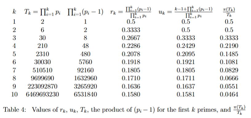
A simple application is the following upper bound for the density of primes by counting the number of coprimes to a given set of prime numbers and their combinations in a certain interval. Let ${ p_1, p_2, \dots, p_{k} }$ be the first ${ k }$ prime numbers. The total number of rows corresponds to the product ${ T_k = \prod_{i=1}^{k} p_i }$ , which is the period over which all combinations of modulus values occur.

Total number of combinations:
$\displaystyle T_k = \prod_{i=1}^{k} p_i$
Number of combinations with no null values:
$\displaystyle \prod_{i=1}^{k} (p_i - 1)$
Number of combinations with at least one null value:
$\displaystyle T_k - \prod_{i=1}^{k} (p_i - 1)$

At the end a simple lemma, that can be easily understood based on the moduli values of the clocks.

Lemma 3 If ${a}$ and ${b}$ are coprime with each other, then their sum ${a + b}$ is coprime to ${a}$ and ${b}$ .

Proof: The remainders (moduli, seconds hands) associated with the prime factors of ${a}$ become zero only at multiples of ${a}$ . Similarly, for ${b}$ , the remainders become zero at multiples of ${b}$ . However, since the sum ${a + b}$ is not divisible by either ${a}$ or ${b}$ , it follows that the remainders for the prime factors of both ${a}$ and ${b}$ are never zero. $\Box$

An upper bound for the primes and density of certain coprimes

Let ${ p_1, p_2, \dots, p_k }$ be the first ${ k }$ prime numbers. The total number of possible combinations of moduli across all rows from 1 to ${ T_k = \prod_{i=1}^{k} p_i }$ is given by ${ T_k }$ . The number of combinations in which all moduli are non-zero is given by ${ \prod_{i=1}^{k} (p_i - 1) }$ . The ratio of these non-null combinations to the total combinations is ${r_k = \frac{\prod_{i=1}^{k} (p_i - 1)}{\prod_{i=1}^{k} p_i}}$ .

Lemma 4 The number of primes in the interval from ${1}$ to ${ T_k = \prod_{i=1}^{k} p_i }$ is at most ${k-1+\prod_{i=1}^{k} (p_i - 1)}$ and the ratio of prime numbers is at most: ${u_k = \frac{k-1+\prod_{i=1}^{k} (p_i - 1)}{\prod_{i=1}^{k} p_i}}$ .

Proof: If the prime number is among the first ${ k }$ primes or the first ${ k }$ primes do not divide it (i.e., all moduli are non-zero), then a number could be prime. If these conditions fail, the number is not prime. However, ${ p_k }$ can still be divisible by a prime with ${ i > k }$ , making ${ u_k }$ a measure of how far this upper bound is from being tight. $\Box$

Let us remark that the bound exactly determines the number of coprimes to any of the composites formed of the first ${ p_k }$ primes in the given interval. In other words all numbers that are not covered must either be primes themselves, greater than ${ p_k }$ , or they are composites of primes greater than ${ p_k }$ . Table 4 below shows the number of combinations and upper bounds for the numbers of primes that one can achieve with this method for combinations of up to 10 primes. We compare it to the known number of primes in the interval.

Visualization of Primes as Complex Exponentials

This section presents a visualization of prime numbers represented as points on concentric circles in the complex plane. Each circle’s radius is proportional to a prime number, and the points on the circles are given by the formula:

$\displaystyle z_i(t) = p_i \exp(2 \pi i t/p_i)$

where ${ p_i }$ is the ${i}$ -th prime number, and ${ t }$ is a parameter that varies.

In the provided plot (Figure 1), the first 10 prime numbers are used, with each prime ${ p_i }$ corresponding to a circle of radius ${ p_i }$ . For a fixed value of ${ t = 30 }$ , the points ${ p_i \exp(2\pi i t)/ p_i }$ are plotted on their respective circles.

Example: ${ t = 30 }$

Consider the example where ${ t = 30 }$ . The points on the circles are determined by:

$\displaystyle z_i(30) = p_i \exp(i \cdot 30 \pi / p_i)$

For each prime ${ p_i }$ , this expression results in a unique point on the circle of radius ${ p_i }$ . The plot shows these points in red, illustrating their positions at ${ t = 30 }$ on the respective circles.

This visualization highlights the rotational symmetry and the behavior of primes when represented as complex exponentials, offering an intuitive geometric interpretation of primes in the complex plane.

It can be observed that the points travel at the same speed on the circles.

Lemma 5 The points ${p_i}$ on the circles travel at a uniform speed.

Proof: The circumference of a circle is ${2 \pi p_i}$ and the points complete a full revolution every ${\pi}$ iterations. Thus, the speed remains the same, irrespective of the circle. $\Box$

From the theory of cycles in the prime clockwork the following lemma be easily observed

Lemma 6 Given an integer ${t}$ positive zeros of the functions ${\phi_{p_i}(t) = p_i \exp{i 2\pi t/p_i}}$ are the prime factors of ${t}$ .

Remark 3 The x-axis crossings of a prime clock with radius 1 can be used as an equation that needs to be satisfied when ${t}$ is integer.

Lemma 7 A number ${p_{i+1}}$ is prime, if and only if ${p_{i+1}}$ is the minimum ${t}$ such that ${\phi_1(t) = (1,0)}$ , and for the preceding primes ${p_1, \dots, p_{i-1}}$ it holds ${\phi_{p_j}(t)/p_i \neq (0,1)}$ .

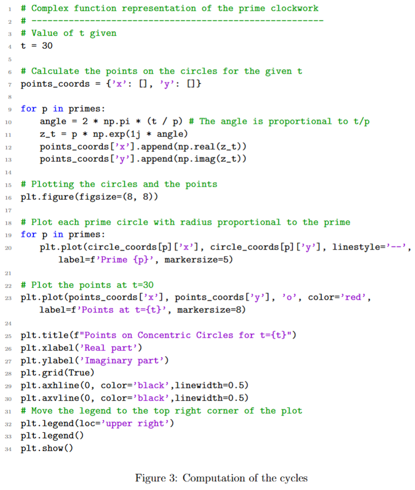
The visualization of integers using the modulus of prime numbers as positions on orbits around the origin offers an intuitive yet comprehensive representation of the prime clockwork. This echoes the earlier metaphor of gears and intertwined cogwheels introduced at the beginning of this essay. Even more captivating is witnessing these wheels in motion. To bring this concept to life, we’ve provided a graphical demonstration powered by a small Python program with interactive source code, available at the following link:

https://trinket.io/pygame/b4608620d3e0?showInstructions=true The program that produced the static plot of the example we provided at the end of our essay. You can change the integer parameter t and get different configurations of the prime clockwork from which all moduli (prime) values and prime factors can be seen in a single view.

Grand Cycles of the Primes

Share this:

Leave a comment Cancel reply